This page describes browser (tree view) functions that are available in the Results environment. A couple of these functions are also available from the command ribbon.
Highlight Items from the Browser
When you click a part in the browser, all of the items associated with the part, based on the current Selection  Select option, are highlighted in the display area. For example, if the selection method is set to elements, clicking a part in the browser will select all of the elements within that part. Then, any operation associated with the selection can be performed, such as Results Inquire Inquire Element Information.
Select option is set to Loads and Constraints. When a contact entry is selected in the browser (either the Default or a particular pair) what is highlighted in the model depends on the analysis type and contact type. See Table 1 for details.
| Table 1: Selecting a Contact Entry in the Browser | ||
|---|---|---|
| Analysis Type | Contact Type | |
| Bonded or Welded | Surface or Edge Contact | |
| Linear | See Note 1. | Nodes connected with contact elements are selected. |
| Nonlinear | See Note 2. | Nothing is selected. |
| Thermal | See Note 1. | Nothing is selected. |
| Electrostatic | See Note 1. | Not applicable. |
- Nodes are selected when any of the following conditions are true:
- Nodes that are smart bonded are selected when the Default or any contact pair is clicked.
- Nodes that are connected together (not smart bonded) are selected if a contact pair other than Default is clicked.
- Nodes that are connected together (not smart bonded) are selected when Default is clicked if smart bonding is also present in the model.
- Nodes that are connected together (not smart bonded) are selected if a contact pair other than Default is clicked.
3D Visualization of Elements
When beam, plate/shell, or 2D elements are included in the analysis, the parts can be displayed or rendered as the 3D geometry instead of the line or planar geometry. This can be done by right-clicking on the heading for that part in the browser and selecting the 3D Visualization command. Table 2 and Figure 1 provide additional details. In all cases, only the nodes and elements on the original mesh can be selected; the fictitious nodes and elements created to show the 3D shape cannot be selected. Loads and boundary conditions are shown at the original mesh.
| Table 2: 3D Visualization | ||
|---|---|---|
| Element Type | Applicable Analysis Type | Notes |
| Beam | Linear and Nonlinear | Cross section shown with 3-D visualization. Beam elements can only be visualized if the cross-sectional properties were defined using the AISC 2001 or 2005 cross-section library or using one of the pre-defined User Defined shapes (wide flange beam, channel, and so on). |
| Plate or Shell | Linear and Nonlinear | Thickness shown with 3-D visualization. |
| 2-D axisymmetric | all | Cross section shown revolved around the Z axis with 3-D visualization. |
| 2-D planar | all | Thickness in -X direction shown with 3-D visualization. |
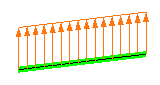 (a) Beam element with loads. A beam element mesh is simply a straight line; the cross sectional properties are treated analytically. |
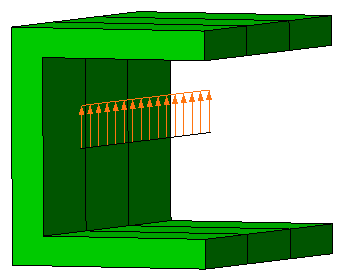 (b) With 3D Visualization active, the actual cross sectional shape is shown. Note how the loads are still shown on the original elements. |
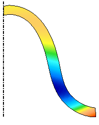 (c) 2D axisymmetric model. Analytically, the analysis treats the model as if revolved around the Z axis. |
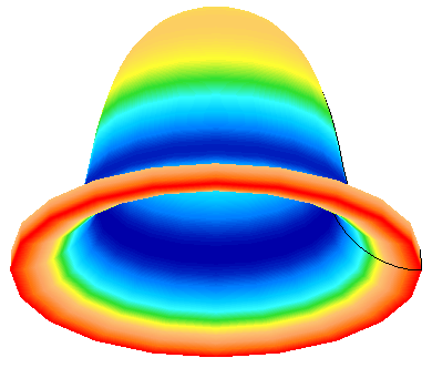 (d) With 3D Visualization active, the 2D mesh and results are shown in their 3D form. The results are the same around the perimeter, so vector results are interpreted as being relative to the Z axis. For example, a true representation of the Y displacement would show a positive value on one side of the model and a negative value on the opposite side. Instead, the Y displacement should be interpreted as the displacement component away from the rotation axis. (A better suggestion is for you to create a cylindrical coordinate system and view the results in terms of radial, tangential, and axial. See the page Setting Up and Performing the Analysis: Using Local Coordinate Systems.) |
| Figure 1: Examples of 3D Visualization | |
 Options Results 3D Element Visualization to control what rendering is performed when the Results environment is launched. See the page Results for details.
 Presentations
The Presentations branch of the browser contains the different views for the current model. The thing to keep in mind is that each presentation is a separate window. To switch between the different presentations/windows, either click the presentation's name in the browser or use the Window pull-down menu and choose the appropriate window. To close a presentation, switch to it and click the X to close the window.
A presentation/window can be either a contour presentation which shows a result by colorizing the model, or a graph/curve which plots the result of selected nodes over time or load cases.
The name of the presentation (shown in the browser and in the window's title bar) only represents the name when the window was created. By using the pull-down menus, the displayed result can be set to anything. Thus, the default Stress presentation may actually be showing a displacement result when changed.
Once a presentation/window is set up with special settings that you want to save for future use, right-click the presentation name in the browser and choose either Save with Model or Save with System.
- A presentation that is Saved with Model will be listed in the saved presentations list only with the original model. The presentation will not be listed with a different model.
- A presentation that is Saved with System will be listed in the saved presentations list when any similar model is opened. For example, a presentation for heat transfer analysis will only be listed when viewing the results of another heat transfer analysis; it would not be listed when viewing the results of a stress analysis.
Mirror Planes
Any model can be mirrored about a maximum of three planes. This is most often used in a symmetry analysis to create a display of the full model. For example, Figure 2 shows the analysis of a symmetric frame. A full display is created in the Results environment to show the complete frame for the report.
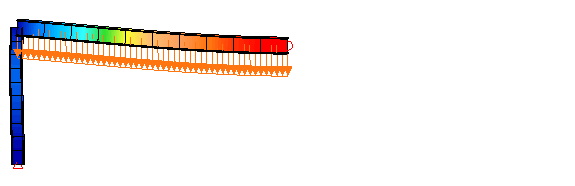 (a) This is the complete model that was analyzed. The analyst took advantage of symmetry and analyzed half of the model. |
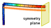
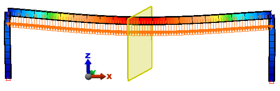 (b) The results are reflected about the mirror plane (the yellow rectangle) to create an image of the full model. The mirror plane can be optionally shown or hidden. |
| Figure 2: Mirror Planes |
The model can be mirrored by right-clicking on the appropriate entry in the Mirror Planes branch of the browser for the current presentation and choosing Activate. To remove the mirror operation, right-click the appropriate plane and clear Activate. To position the mirror plane along the normal direction, right-click and choose Edit Offset. The Offset Distance is the coordinate of the mirror plane, where a positive value is along the positive X, Y, or Z axis normal to the plane. Activating multiple mirror planes will mirror the original model and all the reflections created by other mirrors. For example, a one-eighth symmetry model can be mirrored about the XZ plane to represent a 1/4 symmetry model, which can be mirrored about the YZ plane to represent a 1/2 symmetry model, which can be mirrored about the XY plane to represent the full model. The order of activating the mirror planes is not important.
To show or hide the yellow mirror plane rectangle, right-click the appropriate plane and select or clear Visibility.
The transparency of the mirror plane can be adjusted by using Results Options View Settings Transparency Level, or by right-clicking on any mirror plane entry in the browser and choosing Transparency Level. All mirror planes use the same transparency.
- Only nodes and elements in the original model can be selected. They cannot be selected on the mirrored sections.
- Hiding elements in the model will update all the reflections.
- When a model is sliced and mirrored, the slicing operation is performed first. Thus, all mirrored reflections receive the same slice.
- The results are the same on each side of the mirror plane. This affects vector results the most, such as X, Y, Z displacements. For example, if Figure 2 is showing the X displacement, then the value on one side of the mirror plane would be negative and positive on the other side of the mirror plane. Instead, the same negative displacements are shown on both sides of the mirror plane. Such results should be interpreted as being relative to the mirror plane.
Slice Planes
See the paragraph Slice Planes on the page Display Options for working with slice planes.
Annotations and Labels
The text that appears in the display area is an annotation. You can Add new annotations to the current presentation, and Edit or Move existing annotations. Right-click on the Annotations branch in the browser (or on one of the existing annotations) to access a context menu. When using Add or Edit, the Annotation dialog box appears. The sections are as follows:
-
Annotation text: Type the text to show in the display area. Use the bump-out arrow
 to enter model-specific information, such as the filename, load case number, and so on. Multiple lines can be created either by using the <Enter> key while typing the text, or by adding the new line code (either with the bump-out menu or by typing \n). The Font button is used to format text for the entire annotation (font type, size, color, and so on) using a standard Windows Font dialog box. Some letters and characters may be clipped-off when using italics, depending on the font type.
 - Description: Enter a short description to identify the annotation in the browser.
- Preview and text justification: Specify the point in the annotation that will be the basis of text placement in the display area. When adding a new annotation, click the OK button to close the dialog box, then left-click in the display area to anchor the text at the clicked location. The mouse-click location can indicate the upper, lower, left, or right corners or midpoints of the text bounding box, depending upon the text justification radio button selected. In addition, if Annotation Center is chosen, then the annotation is placed in the display area with the horizontal and vertical center of the text at the mouse-click location. The annotations are anchored to the screen, not to the model. Therefore, annotations will not move if you zoom, pan, rotate, or choose a different model view.
Saved Presentations
The Saved Presentations branch of the browser accesses the default presentations and your saved presentations. Right-click and choose Activate to open the corresponding presentation. Note how this loads the window into the Presentations branch of the browser.
Other Tools Import Presentations. Filter Modules
The Filter Modules branch of the browser is used to set selection filters. A selection filter is used to make it easier to select results of interest while not selecting other items. For example, to sum the heat flow through all the convection faces, use a filter as follows:
- Change the display to show the convection loads on the model (Results Contours Other Results Applied Loads Convection Coefficient).
- Right-click the Filter Modules entry in the browser and choose Add Selection Filter: Current Result. This will give a pop-up dialog.
- Set the Minimum Value and Maximum Value as needed for the filter. If only one value is set, then the filter will be all values up to the maximum or all values above the minimum.
- Change the display to the heat rate (Results Contours Heat Flow Heat Rate Through Face).
- Since heat flow rate needs to be selected by selecting the faces, set Selection Select Faces. Also, use Selection Shape Rectangle to make choosing the faces easier.
- Since the heat out of one face is equal and opposite to the heat flow into the adjacent face, turn the smoothing off (Results Contours Settings Smooth Results should be unchecked).
- Drag a box around the entire model. Only the faces that fit the filter will be selected. From this step, use Results Inquire Inquire Current Results and set the Summary pull-down to Sum. The total heat flow will be display.
Contact Diagnostic Probes
The Contact Diagnostic Probe is used in a nonlinear stress analysis with surface to surface contact to track down areas of contact difficulties. When activated and when a contact problem occurs, the diagnostic probe will appear on the model, and the contact pair is identified in the tree. Two probes per contact pair can appear on the model, one for each diagnostic described below.
The following types of problems will appear in the probe. These are results, so the probe will only appear when the step converges and writes the results.
- Penetration indicates that the contact elements have fully compressed and the two surfaces are now passing through each other (separation less than zero). If this behavior is undesirable, try increasing the contact stiffness, the contact distance (to give a larger cushion), or both values. Remember that the contact elements are essentially springs; they must compress some finite distance to develop a contact force. Thus, a contact distance of zero will require penetration to develop a force.
- Chatter indicates the status of the contact elements (opened or closed) is changing from iteration to iteration. Chatter requires more iterations or reduced time steps to converge, both of which will add to the analysis runtime. Thus, reducing the chatter will be beneficial. At high chatter levels, remeshing the model to have a more uniform mesh is the best solution. Another solution to chattering is to reduce the contact stiffness (softer impact). Also, if the chattering is occurring because the point of contact is shifting from one element to an adjacent element and back, then extending the contact sides can be beneficial. The following levels are shown in the Results environment:
- Level 3: The contact element is oscillating between states.
- Level 4: The contact element status is diverging monotonically. Instead of fewer elements changing status on each iteration, more elements are changing status. If the status continues to diverge, the analysis is not likely to continue.
- Level 5: The contact element status is diverging quadratically. If the status continues to diverge, the analysis is highly unlikely to find a solution.
- If the analysis has reduced the time step greatly due to convergence difficulties, it may require many steps before the analysis gets to the next capture rate step and outputs the results. In this situation, you might want to consider doing the following to see the results at intermediate steps:
- Stop the analysis.
- Activate (check the check box) the option under the Analysis Parameters: Output tab to Output results of all time steps.
- Resume the analysis. (Before resuming, make sure the Automate Analysis is not activated under the Options Analysis tab.)