2D Elements

2D elements are 3- or 4-node isoparametric triangles or quadrilaterals which must be input in the global Y-Z plane. Figure 1 shows some typical 2D elements. The element can represent either planar or axisymmetric solids, as illustrated in Figure 2. In both cases, each element node has two translational degrees of freedom. When the element is used to represent an axisymmetric solid or shell, the global Z-axis is the axis of revolution. All elements must be located in the +Y half-plane where Y is the radius axis. Figure 2 illustrates these conventions.

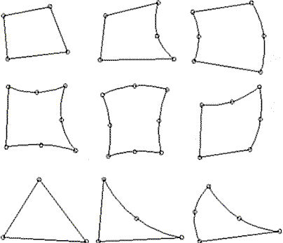
Figure 1: Node Configuration for 2D Elements

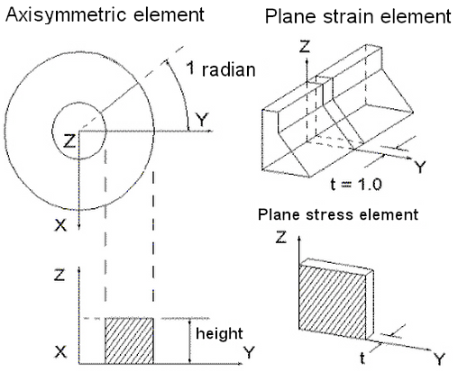
Figure 2: Applications of 2D Elements

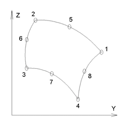
Figure 3: Sample 2D Element

Select Types of 2D Elements

There are three types of 2D elements available for a nonlinear analysis. These can be selected in the Geometry Type drop-down box in the General tab of the Element Definition dialog.

• Axisymmetric: Select this geometry type for elements that model solids with geometric, load and boundary condition symmetry about the Z axis. Negative Y coordinates are not admissible. If a node lies along the axis of revolution (the Z axis) the translation in the Y direction must be constrained. Nodal loads are normalized by the number of radians in a circle (load divided by radians).

  

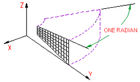
  Figure 1: 2D Axisymmetric Model

• Plane Strain: Select this geometry type to model solids which exhibit no deflection normal to the YZ plane. Since no deflection in the X direction is assumed, a thickness of 1 unit is assumed for the analysis; a thickness can be entered, but this thickness is only used for the 3D visualization in the Results environment. All input loads and results are based on the 1 unit thickness.

  

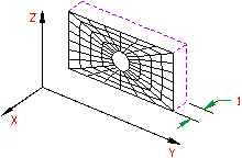
  Figure 2: 2D Plane Strain

• Plane Stress: Select this geometry type to model solids of a specified thickness normal to the YZ plane which exhibit no stress normal to the YZ plane. The constitutive relations are modified to make the stress normal to the YZ plane zero. All loads are distributed uniformly across the thickness.

  

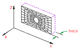
  Figure 3: 2D Plane Stress Model

2D Element Parameters

First, specify the Material model from the list box on the General tab of the Element Definition dialog. Many of the additional input parameters depend on the selected material model. The available material models are grouped in the following categories. (Refer to the appropriate page under the Material Properties page for details on each of the material models.)

• Elastic
  • Isotropic: This material model option is used for parts that will only experience deflections in the elastic region of the stress-strain curve. To use this material model, the parts must have identical material properties in all directions. A single modulus of elasticity and Poisson's ratio will be the requested material properties.
  • Orthotropic: This material model option is used for parts that will only experience deflections in the elastic region of the stress-strain curve. The part may have different material properties in certain directions. Specifically, the material properties may be different in one or more of the three orthogonal directions in a rectangular coordinate system.
  • Variable Tangent: This material model option is used for the analysis of geological materials. This model describes an isotropic material, in which the bulk and shear moduli are functions of the stress and strain invariants.
  • Curve: This material model option is also used for the analysis of geological materials. In this model, the instantaneous bulk and shear moduli are defined by piece-wise linear functions of the current volume strain.
  • Curve with Cut-off: This material model option is similar to the curve material model above, except that in the analysis of some problems, tensile stresses from applied loading cannot exceed the gravity pressure. In this case, you can use this material model to simulate tension cut-off, such as, the material model assumes reduced stiffness in the direction of the tensile stresses which exceed in magnitude the gravity pressure.
  • Temperature Dependent Isotropic: This material model is used to model materials what will only experience deflections in the elastic region of the stress-strain curve but may also experience stress due to a temperature difference.
  • Duncan-Chang Soil: The Duncan-Chang (1970) model is used to simulate soil. It is based on tri-axial soil tests and assumes a hyperbolic stress-strain relation. When using this material model, the Geometry Type cannot be Plane Stress, and the Analysis Formulation on the Advanced tab is set to Material Nonlinear Only.
• Hyperelastic
  • Mooney-Rivlin: This material model is used to model hyperelastic materials such as rubber.
  • Arruda-Boyce: This material model is a hyperelastic material model used to model rubber materials. The implementation follows the Ogden material behavior for volume-preserving deformation modes.
  • Ogden: This material model is used to model hyperelastic materials such as rubber.
  • Yeoh: This material model is used to model nearly incompressible (volume preserving) hyperelastic materials, such as rubber. Only Total Lagrangian analysis formulation is available.
  • Neo-Hookean: This material model is used to model nearly incompressible (volume preserving) hyperelastic materials, such as rubber. Only Total Lagrangian analysis formulation is available.
  • Van der Waals: This material model is used to model nearly incompressible (volume preserving) hyperelastic materials, such as rubber. Only Total Lagrangian analysis formulation is available.
• Foam
  • Blatz-Ko: This material model involves strong coupling between volumetric and non-volumetric parts, such as the bulk modulus, cannot be determined separately as with other hyperelastic material models.
  • Hyperfoam: This material model is used to hyperelastic materials similar to the Ogden material model. This material model will account for the compressibility of the material. This is not applicable to plane strain elements.
• Viscoelastic
  • Viscoelastic Mooney-Rivlin: A viscoelastic variation of the Mooney-Rivlin (hyperelastic) material model.
  • Thermal Creep Viscoelastic: This material model is used to model materials that will only experience deflections in the elastic region of the stress-strain curve but may also experience creep. Creep occurs when a model deflects under a constant load over time. See the paragraph Defining Thermal Properties of 2D Elements for setting up the creep law to use with this material model.
  • Viscoelastic Arruda-Boyce: A viscoelastic variation of the Arruda-Boyce (hyperelastic) material model.
  • Viscoelastic Blatz-Ko: A viscoelastic variation of the Blatz-Ko (hyperfoam) material model.
  • Viscoelastic Ogden: A viscoelastic variation of the Ogden (hyperelastic) material model.
  • Viscoelastic Hyperfoam: A viscoelastic variation of the Hyperfoam material model.
  • Linear Viscoelastic Isotropic: This is a viscoelastic material model in which the material exhibits properties of an elastic solid and a viscous fluid. The viscoelastic properties are based on the Prony series. The properties are equal in all directions (isotropic) and independent of temperature.
  • Linear Viscoelastic Orthotropic: This is a viscoelastic material model in which the material exhibits properties of an elastic solid and a viscous fluid. The viscoelastic properties are based on the Prony series. The properties are different in three perpendicular directions (orthotropic) and independent of temperature.
  • Linear Thermal Viscoelastic Isotropic: This is a viscoelastic material model in which the material exhibits properties of an elastic solid and a viscous fluid. The viscoelastic properties are based on the Prony series. The properties are equal in all directions (isotropic) and dependent on temperature.
  • Viscoelastic Neo-Hookean: This is a viscoelastic variation of the Neo-Hookean (hyperelastic) material model.
  • Viscoelastic Yeoh: This is a viscoelastic variation of the Yeoh (hyperelastic) material model.
  • Viscoelastic Van der Waals: This is a viscoelastic variation of the Van der Waals (hyperelastic) material model.
• Plastic
  • von Mises with Isotropic Hardening: This material model option is used for parts that may experience plastic deformation during the analysis. A bilinear curve will be defined to control the stress-strain relationship.
  • von Mises with Kinematic Hardening: This material model option is also used for parts that may experience plastic deformation during the analysis. A bilinear curve will be defined to control the stress-strain relationship. This material model option is preferred over the von Mises with Isotropic Hardening material model option if the model will undergo cyclical loading.
  • von Mises Curve with Isotropic Hardening: This material model option is used for parts that may experience plastic deformation during the analysis. You will be able to specify a stress-strain curve with multiple data points to control the stress-strain relationship.
  • von Mises Curve with Kinematic Hardening: This material model option is used for parts that may experience plastic deformation during the analysis. You will be able to specify a stress-strain curve with multiple data points to control the stress-strain relationship. This material model option is preferred over the von Mises with Isotropic Hardening material model option if the model will undergo cyclical loading (Bauschinger effect).
  • Temperature Dependent Plasticity: This material model is used to model materials what may experience plastic deformation during the analysis and may also experience stress due to a temperature difference.
• Viscoplastic
  • Thermal Creep Viscoplastic: This material model is used to model materials that may experience plastic deformation and may also experience creep. Creep occurs when a model deflects under a constant load over time. See the paragraph Defining Thermal Properties of 2D Elements for setting up the creep law to use with this material model.
• Drucker-Prager: This material model is similar to the von Mises material models but has the addition of a yielding function. The model assumes that the volumetric strain changes the yielding function. This occurs in materials such as concrete and rock.

Geometry Type: Specify the geometry type using the Geometry Type drop-down box. If using the plane stress or plane strain geometry types, you must define the thickness of the part in the Thickness field of the Element Definition dialog.

Note: The thickness entered for plane strain is only used for the 3D visualization in the Results environment. (See the Browser Functions page.) The input loads and calculated results are based on a thickness of 1 unit.

For the 2D elements in this part to have the midside nodes activated, select the Included option in the Midside Nodes drop-down box. If this option is selected, the 2D elements will have additional nodes defined at the midpoints of each edge. This will change a 4-node 2D element into an 8-node 2D element. An element with midside nodes will result in more accurately calculated gradients. Elements with midside nodes increase processing time. If the mesh is sufficiently small, then midside nodes may not provide any significant increase in accuracy.

Use the Analysis Type drop-down to set the type of displacement that is expected. Small Displacement is appropriate for parts that experience no motion and only small strains and will ignore nonlinear geometric effects that result from large deformation. (It also sets the Analysis Formulation on the Advanced tab to Material Nonlinear Only.) Large Displacement is appropriate for parts that experience motion and/or large strains. (The Analysis Formulation on the Advanced tab should also be set as required for the analysis.)

Tip:

• The displacement at midside nodes is always output. The stress and strain at midside nodes are output only if the user activates the option to output these results before running the analysis. The option is located under the Setup Model Setup Parameters Advanced dialog on the Output tab. (See the Control Output Files page for details.)
• Use the Options Analysis tab and set the Use large displacement as default for nonlinear analyses option to control whether the Analysis Type defaults to small or large displacement.

Control Orientation of 2D Elements

There are two sets of axes for 2D elements: the element axes and the material axes. In this paragraph, the element axes are designated as Elem1 and Elem2, and the material axes are designated as Mat1 and Mat2. Other sections of the documentation may refer to either set as axes 1 and 2.

For a general FEA analysis, you can ignore the element orientation (Elem1 and Elem2). The ability to orient elements is useful for elements with orthotropic material models. This is done in the Orientation tab of the Element Definition dialog. The Method drop-down box contains three options that can be used to specify which side of the element will be the ij side. If the Default option is selected, the side of an element with the highest surface number will be chosen as the ij side. If the Orient I Node option is selected, a coordinate must be defined in the Y Coordinate and Z Coordinate fields. The node on an element that is closest to this point will be designated as the i node. The j node will be the next node on the element traveling counterclockwise (right-hand rule about the +X axis). If the Orient IJ Side option is selected, a coordinate must be defined in the Y, and Z Coordinate fields. The side of an element that is closest to this point will be designated as the ij side. The i and j nodes will be assigned so that the j node can be reached by traveling counterclockwise along the element from the i node.

Once the ij side is determined, the element axis Elem1 is set to be parallel to the ij side. Axis Elem2 is +90 degrees about the X axis. See Figure 1.

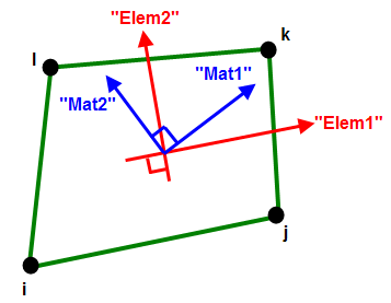
Figure 1: Element Axes and Material Axes

The element axis Elem1 is parallel to the ij edge of the element.

The material axis Mat1 can be offset from the element axis.

Material Axis Direction: When the orthotropic material model is used for 2D elements, three material axes are defined. Material axes Mat1 and Mat2 are in the plane of the element, and Mat3 is parallel to the X axis.

There are two ways to define the material axes from the General tab of the Element Definition dialog. The first is to define a vector using the Y Direction and Z Direction fields. Material axis 1 is parallel to the global vector. Material axis 2 will be the cross-product of the X axis and material axis 1. Figures 2 and 3 illustrate this method. If no value is specified in the Y Direction or Z Direction fields, the value in the Material Axis Rotation Angle field will be used to orient the material axes relative to the element axis Elem1. This is useful if a part was molded from an original sheet into a specific shape. The rotation angle β corresponds to the angle of material axis 1 relative to the element axis 1 of each element. See Figure 4.

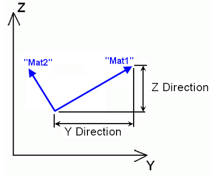
Figure 2: Y and Z Direction Definition of Material Axis Direction

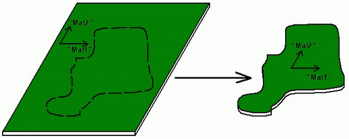
Figure 3: Part Cut Out From Orthotropic Material

Although the mesh will be random, resulting in random element axes, the material axes are consistent.

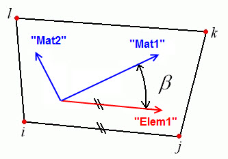
Figure 4: Rotation Angle Definition of Material Axis Direction

Define Thermal Properties of 2D Elements

Thermal Section:

If a 2D element part is using a material model with thermal effects, you must specify a value in the Stress free reference temperature field in the Thermal tab of the Element Definition dialog. This value is used as the reference temperature to calculate element-based loads associated with constraint of thermal growth using bilinear interpolation of the nodal temperatures.

Creep Section:

If a 2D element part is using a material model that includes creep, select the option in the Creep law drop-down box. This selection will be used to calculate the creep effects during the analysis. The creep laws available are as follows:

• No creep: When this option is chosen, no creep effects are included in the analysis.
• Power-law: This option is also known as the uniaxial creep law. The equation is = C ₁ x ^C2 x t ^C3 .
• Garofalo: This option is also known as the hyperbolic sine creep law. The equation is = A ₀ x [sinh(A ₁ x )] ^A2 .
• Double power-law: This option is similar to the power law but with an additional term to produce results closer to experimental results at high stress levels. The equation is = C ₁ x ^{C 2} x t ^C3 + C ₄ x ^C5 x t ^C6 .

where is the effective creep strain rate and is the effect stress. Also refer to the Thermal Creep Viscoelastic Material Properties page for important information on entering the material properties.

For the creep calculations to be calculated on evenly sized divisions of the time step, select the Fixed substeps option in the Time integration method drop-down box. For the creep calculations to be calculated on variable sized divisions of the time step, select the Flexible substeps option. These two methods are based on time hardening and use explicit time integration methods. These methods may become unstable under some loading conditions. When using the Thermal Creep Viscoelastic material model, an additional option will be available in the Time integration method drop-down box: the Alpha-method. This method uses an implicit time integration scheme to improve the creep behavior. This method can be unconditionally stable.

Specify the temperature at which no thermal stress exists in the Stress free reference temperature field.

The Effective option in the Creep strain definition drop-down box is appropriate for an analysis with non-cyclical loading.

During the analysis, the creep calculations will be performed as iterations in substeps of each time step. You can control how many substeps are allowed in a single time step in the Maximum number of substeps field. You can also specify how many iterations can be performed in a single substep in the Maximum number of iterations in a substep field. After each substep iteration, the creep stress and strain will be compared to the previous iteration. If the value is not within the tolerances specified in the Creep strain calculation tolerance and Creep stress calculation tolerance fields, another iteration will be required.

When using a Time integration method of Alpha-method, the Time integration parameter needs to be specified. To use a fully explicit method for the time-integration scheme (but different than the fixed/flexible substeps' explicit method), type 0.0 in the Time integration parameter field. To use a fully implicit method, type 1.0 in the Time integration parameter field. When the Time integration parameter is greater than 0.5, this method is unconditionally stable.

Advanced 2D Element Parameters

Select the formulation method that you want to use for the 2D elements in the Analysis Formulation drop-down box in the Advanced tab.

• If the Material Nonlinear Only option is selected, nonlinear material model effects will be accounted for but all calculations will be performed based on the undeformed geometry. Thus, this formulation is suitable for parts with small strains and no motion. This will be the only option available if the Analysis Type on the General tab is set to Small Displacement.
• The Total Lagrangian option will refer to the initial undeformed configuration of the model for all static and kinematic variables. This formulation is suitable for parts with motion and small strains. Note that the material properties should be in terms of engineering stress and strain.
• The Updated Lagrangian will refer to the last calculated configuration of the model for all static and kinematic variables. This formulation is suitable for parts with motion and large strain. Note that the material properties should be in terms of actual stress and strain.

Next, select the integration order that will be used for the 2D elements in this part in the Integration Order drop-down box. For rectangular shaped elements, select the 2nd Order option. For moderately distorted elements, select the 3rd Order option. For extremely distorted elements, select the 4th Order option. The computation time for element stiffness formulation increases as the third power of the integration order. Consequently, the lowest integration order which produces acceptable results should be used to reduce processing time.

The Stress Update Method is used when the material model (on the General tab) is set to one of the following plastic material models:

• von Mises with Isotropic Hardening
• von Mises with Kinematic Hardening
• von Mises curve with Isotropic Hardening
• von Mises curve with Isotropic Hardening

This controls the numerical algorithm for integrating the constitutive equations (stress/strain law) when the material goes plastic. The options available for the Stress Update Method are as follows:

• Explicit: (Original method). This option uses the explicit sub-incremental forward-Euler method for integrating the constitutive equations. The Explicit option is best used for simple problems, such as simple tension, because the method runs faster. However, it is more sensitive to the loading and time step size.
• Generalized Mid-Point: This option uses an implicit method for integrating the constitutive equations. It reduces the error accumulation and can ensure that the stress updating process is unconditionally stable. Thus, this option is better suited for complicated analyses, such as contact problems and severe plasticity.

The Parameter for Generalized Mid-point input is used when the Stress Update Method is set to Generalized Mid-Point. Acceptable ranges for this input are 0 to 1, inclusive. When the Parameter is set equal to 0, the resulting algorithm would be a fully explicit member of the algorithm family (similar to the Explicit option for the Stress Update Method); however, the solution is not unconditionally stable. When the Parameter is 0.5 or larger, the method is unconditionally stable. When the Parameter is set to 0.5, the solution is known as a mid-point algorithm; when it is 1, the solution is known as the fully backward Euler or closest point algorithm and is fully implicit. A value of 1 is more accurate than other values, especially for large time steps.

The Strain Measurements is used when the Material Model (on the General tab) is set to Isotropic and the Analysis Formulation is set to Updated Lagrangian. The options are used to improve the convergence of the updated Lagrangian method. The options available for the Strain Measurements are as follows:

• Almansi Strain: (Original method). This option uses the Cauchy stress and Almansi strain for the constitutive relation. It is limited to cases of small strain.
• Log-strain: This option uses the Cauchy stress and virtual log-strain (incremental strain) for the constitutive relation. It is acceptable for all cases, including large strain. This is a hypoelastic model, and one drawback is that it works better for incompressible material (Poisson ratio = 0.5) than compressible materials. This is because the shear modulus is assumed to be a constant where as it changes with the varying volume in reality.

If the Allow for overlapping elements check box is activated, overlapping elements will be allowed to be created when the lines are decoded into elements. Overlapping may be necessary when modeling elements. This is especially true for problems confined to planar motion.

For the stress results for each element to be written to the text log file at each time step during the analysis,. activate the Detailed stress output check box. This may result in large amounts of output.

If one of the von Mises material models has been selected, you can choose to have the current material state (elastic or plastic), current yield stress limit, current equivalent stress limit and equivalent plastic strain output at corner nodes and/or integration points at every time step. This is done by selecting the appropriate option in the Additional output drop-down box.

Define Soil Conditions

If the Duncan-Chang material model is chosen, the Soil tab is enabled. Enter the following input as appropriate for the analysis. This input is related to the initial state of the soil; also see the Duncan-Chang Theoretical Description page for information.

• Superimpose hydrostatic pressure When activated, the initial stress is created from a constant hydrostatic pressure entered in the accompanying field. (Hydrostatic pressure in this case is acting equally in all directions, not to be confused with a pressure that increases with depth) The magnitude of the pressure must be greater than 0.
• Superimpose self weight When activated, the initial stress is created from the weight of the modeled soil.
• Reference point on surface Specify an X, Y, Z coordinate. This establishes where the pressure due to the weight of the soil is zero. If the model is a section of soil deep underground, then the reference point can be above the part modeled.
• Coefficient of lateral earth pressure Most soils do not create a true hydrostatic stress (equal in all directions). The stress in the horizontal directions is normally some fraction of the vertical normal stress. The ratio of lateral/vertical stress defines the coefficient of lateral earth pressure. The input should be in the range of 0 to 1.
• Gravitational acceleration To create a stress distribution due to the self weight, enter the gravitational constant and direction in which gravity was acting to create the stress distribution. The direction is normally the same direction that gravity acts in the analysis. However, a different direction can be used if the model represents the soil in a different orientation between the time the initial stress was created and the current orientation of the model. The soil was moved.

Define Damage Analysis Types

If the Material model is Orthotropic and the Geometry Type is Plane Stress, then the Damage tab will be enabled.

The damage model simulates the damage onset and the progressive growth for elastic-brittle orthotropic materials. The model is primarily intended to be used to simulate fiber-reinforced composite materials. See the Damage Theoretical Description page for additional details on the calculations.

The damage model works for Material nonlinearity only and Total Lagrangian Analysis Formulations but not Updated Lagrangian method.

Note: The maximum size for the element in a damage analysis is L_c<=2*EⁱG^c_i/(Xⁱ)², where Eⁱ, G^c_i, and Xⁱ are the Young's modulus, fracture energy, and strengths, respectively, for each of the four damage modes (fiber tension and compression, matrix tension and compression).

The following damage initiation criteria can be selected:

• None no damage calculations are performed.
• Damage initiation Whether and where damage occurs in the part is calculated, but what happens after damage initiation is not calculated. The tensile fiber criterion (f_I), compressive fiber criterion (f_II), tensile matrix criterion (f_III), and compressive matrix criterion (f_IV) are calculated.
• Damage initiation and evolution What happens after damage occurs is calculated. The element stiffness is reduced when damage occurs. In addition to the values calculated above, the tensile fiber damage (d_ft), compressive fiber damage (d _fc ), tensile matrix damage (d_mt), compressive matrix damage (d_mc), and damage energy density (ΔE_D) are calculated.
• Damage initiation and stabilized evolution The previous method is preferred when the effects after damage are required, but the analysis may be unstable when the damage occurs due to the sudden loss of stiffness. Choosing this method adds some viscous regularization (Duvaut-Lions) to help stabilize the solution. Since this is artificial, the minimum amount of viscosity necessary to get a stable solution should be used. After the analysis, compare the damage energy density result with the viscous energy density result. The viscous energy density should be much smaller than the damage energy density in order for the viscous effects to be negligible. In addition to the values calculated above, the viscous energy density (ΔE _V ) is calculated. When this option is chosen, the following input is also enabled in the Viscosity Parameter for Damage Stabilization section:
  • Local Axis 1 (Tension) the viscosity coefficient for the mode of fiber tension (η_ft)
  • Local Axis 1 (Compression) the viscosity coefficient for the mode of fiber compression (η_fc)
  • Local Axis 2 (Tension) the viscosity coefficient for the mode of matrix tension (η_mt)
  • Local Axis 2 (Compression) the viscosity coefficient for the mode of matrix compression (η_mc)

Tip: Use the Material Axis Direction on the General tab to set up the orientation of the material. See the paragraph Controlling the Orientation of 2D Elements above for details.

Basic Steps for Use of 2D Elements

1. Be sure that a unit system is defined.
2. Be sure that the model is using a nonlinear analysis type.
3. Right-click the Element Type heading for the part that you want to be 2D elements.
   Tip: Useful commands for converting 3D models to 2D models are Draw Pattern Relocate & Scale, Draw Pattern Rotate or Copy, and Draw Modify Project to Plane. For example, you may accidentally create a mesh in the XY plane. You can rotate the mesh to the YZ plane using either the Relocate & Scale or Rotate command. Due to round-off, some nodes may have a small X coordinate value that prevents the element type from being set to 2D. In this case, use Project to Plane to snap the nodes exactly to the YZ plane.
4. Select the 2D command.
5. Right-click the Element Definition heading.
6. Select the Edit Element Definition command.
7. In the General tab, select the appropriate material mode in the Material Model drop-down box.
8. Select the appropriate geometry type in the Geometry Type drop-down box.
9. Enter the thickness of the 2D elements if you selected the Plane Stress or Plane Strain option in the Geometry Type drop-down box.
10. If you selected material model that includes thermal or creep/viscoelastic effects, specify the necessary information in the Thermal tab.
11. Press the OK button.