Local Mesh Refinement

Often, critical stresses are limited to one or two small areas of a model. When Global Mesh Refinement is used, the resulting mesh is often finer than necessary because all elements are resized. A more efficient approach is to refine the mesh locally, only where the critical stress regions are. The Local Mesh Refinement command provides a semi-automatic means of performing this targeted mesh refinement on CAD-based models.

Set up the Model

Before performing local mesh refinement, first perform the following steps:

1. Open the CAD model in Autodesk Simulation Mechanical.
2. Set the analysis type to Static Stress with Linear Material Models.
3. Set any special meshing options such as the type of mesh (solid, midplane, plate/shell), refinement points, mesh matching tolerance, and so on.
4. Mesh the model. The Local Mesh Refinement command will not be available for selection until after the model is meshed.
5. Add surface, edge or part loads and constraints to the model. Nodal loads applied to the CAD parts will not be retained during the mesh refinement process.
6. Define the Element Definitions.
7. Define the Material properties.
8. Define the Analysis Parameters.
9. Optionally, do a Check Model or perform the analysis.

Tip:

• Although the model does not need to be meshed prior to Local Mesh Refinement, we recommend you do so to reveal any problems with the model and setup.
• Although it is not necessary to do a Check Model or perform the analysis, we recommended you do so to uncover any problems with the model and setup.

Set up and Run Local Mesh Refinement

1. Click Analysis Mesh Refinement Local Mesh Refinement.
2. If you know the coordinates at the center of the critical stress region, you can type them into the X, Y, and Z input fields. Otherwise, click a vertex on the model surface to select the center point of the refinement region.
3. Type a value into the Effective Radius field to specify the size of the spherical refinement region. An orange sphere appears on the model with a black dot at the center. This is the area where the mesh will be refined.

   

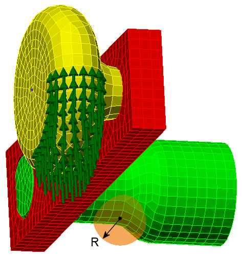
   Figure 1: Local Mesh Refinement Region

4. Click Next.
5. In the Total Iterations field, specify the number of mesh refinement iterations you want to perform. The default is four. The original mesh is analyzed (as meshed in the current design scenario) plus the specified number of refinement iterations.
6. Specify the desired Divide Factor. The local mesh size is divided by this factor for each iteration. For example, if you specify four iterations and a divide factor of 1.3, the resultant relative mesh sizes will be 1, 0.769, 0.592, 0.455, and 0.350 (1/1.3⁴ = 0.350).
7. Click Next.
8. Select the Target Computer (Local or Cloud). Only the Local option is available for the desktop version of Simulation Mechanical.
9. Click Analyze.

New design scenarios are created for each refinement iteration, and the original and refined design scenarios are solved. You will see the effects of the local mesh size reductions for each design scenario as they are being prepared. The following image shows the local mesh refinement for the last iteration of our example model:

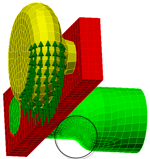
Figure 2: Refined Mesh in Local Mesh Refinement Region

When the solving process is done, a pop-up message indicates that local mesh refinement is finished. Click OK to dismiss the pop-up message and view the results. The original design scenario is displayed in the Results environment, and you can double-click the heading for any of the other design scenarios to view the results of the other iterations.

A graph of the Local Mesh Refinement Result is displayed in the Convergence Plot tab of the Output Bar.

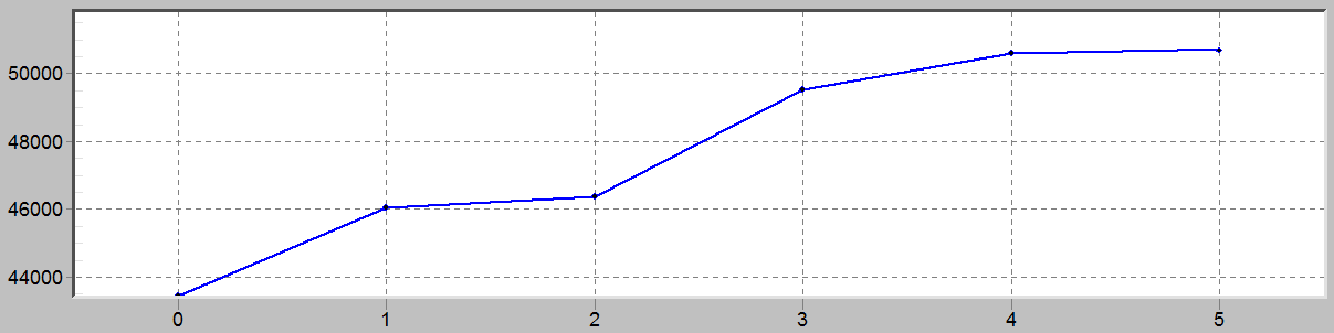
Figure 3: Local Mesh Refinement Result (Convergence Plot)

Customize the Local Mesh Refinement Result Graph

There are two drop-down selection menus at the upper right corner of the Output Bar while viewing the convergence plot, as follows:

• Local Max Result or Global Max Result: Choose whether the data points on the graph are based on the maximum result for the entire model (Global) or only within the mesh refinement region (Local). Due to the effect of the local mesh on the adjacent elements, the elements beyond the refinement region will also be different for each iteration. In addition, the change in stiffness within the refined and nearby elements will affect the stress and displacement results elsewhere in the model.

  It is a good idea to look at the global results to ensure that there are no unanticipated critical stress or displacement magnitudes. However, the most accurate indication of the effect of the local refinement is observed when limiting the plotted result to those from the local refinement region.

• Using the second drop-down selector, choose which result to plot:
  • Von Mises Stress
  • Maximum Principal Stress
  • Minimum Principal Stress
  • Magnitude Displacement
  Note: See the Linear Results page for a description of these results.
• Include internal nodes: By default, the Local Mesh Refinement results do not include the stresses or displacements at internal nodes. This behavior is consistent with the default contour plots in the Results environment. Normally, critical stresses exist at the outside surfaces of structures. Thermal stresses are the exception. Stresses due to thermal expansion or contraction can be greatest within the volume of a solid, not necessarily at the surface.

  When peak stresses might be greatest it the interior of a model, activate the Include internal nodes option. The Local Mesh Refinement graph will consider exterior and interior nodes. For consistency between contour plots and Local Mesh Refinement results, also activate Results Options View Show Internal Mesh within the Results environment.

  Note: For conventional structural analyses, peak stresses may be calculated in the interior of a part due to poor mesh quality or distorted elements. In such cases, it is safe to exclude the internal nodes from the Local Mesh Refinement results. It is only important to consider internal nodes for the special cases where peak stresses can legitimately occur below the surface of the parts.

Context Menu

A context menu appears when you right-click in the graph display area. This menu contains many options for customizing the appearance of the graph and exporting the graph to various image file formats. The graph options behave the same as for graphs in the Results environment. So, if you are familiar with customizing and exporting those graphs, the mesh convergence graphs are the same. Most of the customization options are self-explanatory.

Interpret the Convergence Plot

The Local Mesh Refinement graph is based on smoothed results. Therefore, the graph agrees with the default stress contours viewed in the Results environment. The command Results Inquire Inquire Maximum Results Summary will generally show higher stress values, because this command lists unsmoothed stresses.

Ideally, the change in results will become insignificant in the latter iterations. When the element size is too coarse, stresses are not accurately captured. As the elements become finer, the stress results typically increase. Once the mesh is fine enough to produce accurate stress results, further decreasing of the mesh size produces a diminishing effect on the results.

Displacement results are usually less sensitive to mesh size and quality than the stress results are. Therefore, differences between displacement results may not be very significant even for relatively coarse meshes. Note the values along the vertical axis of the graph. The scale of the Y-axis can exaggerate the difference between the values.

Distorted elements can cause anomalous high-stress results. In such cases, the graph will look like the results are not converging. A single point of concentrated high stress (that is, a singularity), which is not explainable by the geometry or loads, can often be safely ignored. The stress results in the critical regions may be reasonably converged despite a graph that does not level off. It is the responsibility of the engineer or stress analyst to determine when it is safe to disregard results singularities.

Create a Local Mesh Refinement Report

When viewing the convergence plot, there is a Save… button at the right side of the Output Bar. Click this button to save a local mesh refinement report in ASCII text format. A Save As dialog box appears. Enter a name in the File name field and use the Save as type drop-down selector to choose what file extension you want (*.dat or *.txt). In either case, the contents of the file will be plain ASCII text. The resultant file can be opened in Notepad or any similar text editor.

Contents of the Saved File:

• Coordinates of the refinement region Center point
• Radius of the refinement region
• The Divide Factor that you specified
• Target computer
• A table listing the results for all iterations. There are four sections to the table, one for each available type of result:
  • Von Mises stress
  • Maximum principal stress
  • Minimum principal stress
  • Displacement magnitude

  Each result type tabulation includes the following columns:

  • Iteration number
  • Divide Factor (cumulative)
  • Design scenario number
  • Global maximum result: The label suffix will say (Including Internal) when the Include internal nodes option was activated for the saved results.
  • Node number where the global maximum result occurs
  • Local maximum result: The label suffix will say (Including Internal) when the Include internal nodes option was activated for the saved results.
  • Node number where the local maximum result occurs