The results options discussed on this page are located under one of the following three ribbon tabs:
- Results Contours
- Results Inquire
- Results Options
Load Case Options
The following are the definitions and uses of the buttons available in the Load Case Options panel. This submenu will only be available if the current model has multiple load cases.
Load case and time step in a dynamic analysis can be thought of as equivalent terms: they represent one set of results due to particular load combinations or at a particular instant in time.
- First: This command will cause the loads and results of the first load case to appear.
- Previous: This command will cause the loads and results of the previous load case to appear.
- Middle: This command will cause the loads and results of the middle load case to appear.
- Next: This command will cause the loads and results of the next load case to appear.
- Last Results: This command will cause the loads and results of the last analyzed load case to appear. The last load case that has results. If the analysis is stopped before reaching the end (or if the analysis is ongoing), then the last analyzed load case and the last requested load case will be different load case numbers.
- Last Requested: This command will cause the loads of the last load case to appear. If the analysis has reached the end, then the results will be available also.
- Set: This command will access a screen in which you can specify a specific load case for which to view the results.
- Automatic Advance: Some analysis types output the results of a load case as soon as they are calculated, making them available for reviewing. Nonlinear and transient heat transfer analyses are examples of when you should review the results throughout the analysis to confirm that the model is set up and proceeding as expected.
When the Automatic Advance command is activated, the results will update when new results become available. If the command is deactivated, either by turning it off or by choosing a different load case, then new results will not be displayed when they are calculated.
- Analysis in Progress: For analyses that utilize the Automatic Advance command, this menu item indicates whether the analysis is in progress (menu is checked) or not in progress (menu is not checked). Some functions are disabled while the analysis is ongoing, such as making changes to the model and exiting from the software.
The analysis is considered to be ongoing whenever the analysis window is opened, even if the analysis itself has completed.
Spectrum Component
When viewing the results of a Response Spectrum analysis and the calculation method is either the NRC Reg. Guild 1.92 or Modified Procedure, then the Results Options Analysis Specific Spectrum Component is available. Individual results are given for each spectrum loading direction (the X, Y, Z direction factors in the Analysis Parameters) and each natural frequency. The Spectrum Component command sets which loading direction is shown, and Results Contours Load Case Options sets which natural frequency is shown.
Resultant
This command will only be available for a response spectrum, random vibrations, and dynamic design analysis method (DDAM) analyses. This will be active by default. The display will show the resultant of all the natural frequencies used in the analysis. To view the individual components of the natural frequencies, deactivate this command. Each natural frequency will now be displayed as a separate load case.
- The Resultant is often an SRSS (square root sum of the squares) of the results of the individual modes. Therefore, the sign of the result is lost (all values become positive). Therefore, the magnitude of the result may have some significance, but information about direction is not available.
- For example, take the maximum principal stresses of 300 and 450 in modes 1 and 2, and a minimum principal stress of -14000 and -12500. The negative sign indicates compression for the minimum principal stresses. The SRSS of these would be 541 and 18770, respectively. Since the negative sign is lost, the minimum principal stress appears to be larger than the maximum principal stress.
Response Type
This command will only be available for a frequency response analysis. You will have the option of viewing the in-phase, out-of-phase or SRSS (square root sum of squares) results for each applied frequency.
Smooth Results
- The following discussion about smoothing the results is based on the default settings. The Smoothing Options command has many settings that affects the following behavior of the Smooth Results command, such as:
- the type of smoothing operation (show the mean value, show the range between results at a node, and so on)
- smoothing between different parts in the model
- the order of the arithmetic operations (smooth before or after calculating the final result)
The Smooth Results command is used to produce a smoother display of the displayed model, without abrupt transitions between colors. For results that are element based (such as stress), the values at the nodes are calculated independently in each element. Therefore, a step change or discontinuity can exist across an element boundary. The differences are a natural result of the FEA process. To some degree, the actual stress may be close to the average of all the different stresses at the node. This is what the Smooth Results command does: it averages the results between adjacent elements and displays that average at the node.
This approach is reasonable provided that the model is continuous. If the model has a step change (such as a change in plate element thickness), then the stresses at the boundary between the different parts should not be averaged (and are not averaged by default).
If the Smooth Results command is not activated, the data will be viewed in the raw form, so each node will have multiple results (one result for each element attached to the node).
For results that are nodal based (displacement, temperature, velocity, and so on), there is only one value at a node, so the Smooth Results command has no effect.
Smoothing Options
When this command is selected, the Smoothing Options dialog will appear.
- Smoothing Function: This drop-down box will allow you to control the value that is used for the smoothed value at each node.
- None: This option will remove the smoothing from the model. This is the equivalent of deactivating Results Contours Settings Smooth Results.
- Maximum: This option will use the maximum value from all the elements that meet at each node and use that value for the smoothing at that node.
- Mean: This is the default smoothing method. This will take the average of the values from all the elements for each node and use that value for the smoothing at that node.
- Minimum: This option will use the minimum value from all the elements that meet at each node and use that value for the smoothing at that node.
- Range: This option will take the difference of the minimum and maximum values from all the elements that meet at each node and use that value for the smoothing at that node.
- Sum: This option will add up the values from all the elements that meet at each node and use that value for the smoothing at that node.
- None: This option will remove the smoothing from the model. This is the equivalent of deactivating Results Contours
- Smooth Across Part Boundaries: If this check box is activated, the values will be smoothed at the nodes that are shared by elements in different parts of an assembly. You can limit the boundaries that will be smoothed across by deactivating one of the options below.
- Smooth Across Element Type Boundaries: If this option is active, the values will be smoothed at the nodes that are shared by elements of different types. This command applies only to element types of similar geometry types. For example, if this option is active (and the Smooth Across Geometry Type Boundaries check box is not activated) the results will be smoothed across two parts consisting of bricks and tetrahedrals or plates and membranes or trusses and beams. The results will not be smoothed across two parts consisting of beams and bricks.
- Smooth Across Geometry Type Boundaries: If this check box is activated, the values will be smoothed at the nodes that are shared by elements of different geometry types. There are three geometry types: solids (bricks and tetrahedrals), planar (2D, plates, membranes and composites), and line (trusses and beams).
- Prohibit Smoothing Across Break-Angles Larger Than: If this check box is activated, the results will not be smoothed at any node shared by two elements with a break-angle larger than the value entered in the field below this option. The break-angle is the angle between the vectors normal to the faces of the elements. For example, if two plate elements lie in the same plane, the break-angle is 0 degrees. If two plate elements meet at an edge of a cube, the break angle is 90 degrees.
- Consider Element-Local Coordinate System: If this check box is activated, the angle between the local 1, 2, and 3 axes will be used instead of the break angle. If the angle between the local 1 axis of one element and the local 1 axis of an adjacent element is greater than the value prescribed in the field above this option, the results will not be smoothed at this node. The same effect will occur if the angle between the local 2 or 3 axes of adjacent elements are greater than the specified value.
- Smooth Before Applying Operators: Some secondary results, such as von Mises stress and principal stress, are the result of a calculation based on other results. When these secondary results are smoothed, there are two ways that the smoothing could be applied to the calculation. One option is to smooth the base results that are used in the equation, and then calculate the final result. This gives one final result. The second option is to calculate the secondary result based on the unsmoothed base results which gives N number of secondary results and then apply the smoothing to the N number of secondary results to give one final result.
When the Smooth before applying operators box is not activated, the calculations are made in the following order:
- Retrieve the base results (for example, Stress Tensor).
- Translate reference frame, if requested.
- Apply operator or equation using the base results to give N results.
- Smooth N results per the smoothing function to give one final result.
When the Smooth before applying operators box is activated, the order of the last two calculations is swapped.
- Retrieve the base results (for example, Stress Tensor).
- Translate reference frame, if requested.
- Smooth the base results per the smoothing function.
- Apply operator or equation using the smoothed base results to give one final result.
This can yield significantly different results wherever the base result has a sharp change across multiple elements at a single node. For example, take the following results from a 2D stress analysis. The two elements are connected at the common node number 21.
Stress Value Element 10, Node 21 Element 11, Node 21 Mean Value Stress YY 1,635.8 362.5 999.2 Stress ZZ 425.7 8.8 217.3 Shear YZ -294.4 534.1 119.9 von Mises 1,555.9 992.0 1,274.0 Using the mean smoothing function and for smoothing after applying the operators (Smooth before applying operators is unchecked), the final result for the calculation of the von Mises stress would be the average of the two individual von Mises stresses, or 0.5*(1,555.9+992.0) = 1,273.9. For smoothing before applying the operators, the final result would be the von Mises equation using the mean value of the stress tensors, or
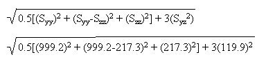 = 933.6. This hypothetical model has a large change in stress between adjacent elements and the mesh should be refined. In areas with no large discontinuity in the base results between neighboring elements, Smooth before applying operators should cause no large change in the plotted result. When plotting scalars or individual components of tensors or vectors, the Smooth before applying operators check box will have no visible affect at all other than a small performance penalty.
 For the factor of safety calculation, imagine a yield stress of 2000. For smoothing after applying the operators, the factor of safety would be the average of the individual factors of safety, or 0.5*(2000/1555.9+2000/992.0) = 1.65. For smoothing before applying the operators, the stress components are smoothed first, then the one von Mises stress is calculated, then the one factor of safety value is calculated, or 2000/933.6 = 2.14.
For another example, take a hypothetical model where heat is flowing directly away from a nodal heat source at an equal rate, in opposite directions through two different elements using the node. (Keep in mind that heat flux is a vector result.) Realizing that magnitude is an operation on individual vector components, mean heat flux magnitude would be some positive value X when smoothing after applying operators (calculate the magnitude of each vector, then average) but would be zero when smoothing before applying operators (mean of two equal, opposing vectors, then calculate the magnitude).
The table below summarizes these examples.
Smooth after applying operators Smooth before applying operators von Mises stress - Calculate the von Mises stress σvMn for each node on each element.
- Smooth the individual von Mises calculations σvMn. For mean smoothing,
- Smooth individual stress tensors for each node on each element.
- Calculate the von Mises stress from
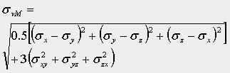
where all the six stress components are smoothed.
Factor of safety - Calculate the von Mises stress σvMn for each node on each element.
- Calculate the factor of safety for each node on each element,
- Smooth the factors of safety. For mean smoothing,
- Calculate one von Mises stress value using the smoothed tensor stresses (steps 1 and 2 above).
- Calculate the factor of safety from the one von Mises stress
Magnitude of heat flow vector - Calculate the magnitude of each vector.
- Smooth the individual magnitudes.
- Smooth all of the vectors for each node for each element.
- Calculate the magnitude.
Similarly, Smooth before applying operators can have a large effect when using the Absolute Value operator with base values of different sign at a single node, or when using the von Mises operator on tensors that have similar principal values but different principal directions.
Tip: If the Smooth before applying operators option is grayed out, then this option is not applicable to the current result type.
Absolute Value
If this command is activated, the absolute values of the contour will be displayed. If you are using the Smooth Results command, the absolute values will be used for the smoothing at each node.
Maximum Value
If this command is activated, the elements will be contoured according to the node with the highest stress display value. This can be used along with the Absolute Value command. This option will not be available if the Smoothing Options command is active.
Factor Of Safety
If this command is activated, the factor of safety for the selected stress contour will be shown. The factor of safety is the ratio of the allowable stress to the actual stress. A factor of safety of 1 represents that the stress is at the allowable limit. A factor of safety of less than 1 represents failure. A factor of safety greater than 1 represents an acceptable analysis. The allowable stresses can be assigned on a per part basis by selecting the Set Allowable Stress Values command.
See the section Smoothing Options for important information about how the Smooth before applying operators option will effect the factor of safety calculation.
Set Allowable Stress Values
When this command is selected, the Allowable Stress Values dialog will appear. Each part will be listed in a separate row. You can either specify a value in the Allowable Stress column or press the Load Yield Stress or Load Ultimate Stress buttons to load the values from the material library. If no value exists, the allowable stress will be set to 0. Any parts for which the allowable stress is set to 0 will be excluded from the factor of safety calculations.
Show Displaced Model
If this command is activated, the displaced model will be shown at the default scale. You can modify the scale using the Displaced Model Options command.
Displaced Model Options
When this command is selected, the Displaced Model Options dialog will appear.
- Displaced Model section
- Show Displaced Model: Activating this option will allow you to show the deflected shape of the model due to the loading. You can control the scale of the deflected shape using the Scale Factor section. Any result contour will still be displayed on the displaced shape.
- Scale Factor section
- As an Absolute Value: If this option is selected, you will control the scale of the deflections according to a scale factor. This value can be entered in the Scale Factor field. The model will be automatically scaled in the display area to correspond to the specified scale factor when the <Enter> or <Tab> key is pressed.
- As a Percentage of the Model Size: If this option is selected, you will control the scale of the deflections according to a percentage of the model size. This percentage can be controlled by either entering a value in the Scale Factor field or using the slider bar. The model will be automatically scaled in the display area to correspond to the specified scale factor when the <Enter> or <Tab> key is pressed.
- Show Undisplaced Model As section
- Do Not Show: Select this radio button if you do not want the undisplaced model to be displayed.
- Mesh: Selecting this radio button will display the mesh of the unloaded model to use as a reference frame for the deflected shape. The undisplaced shape will not be shaded.
- Mesh on Top of Displaced Model: Selecting this radio button will force the mesh lines of the undisplaced shape to be shown on top of the shaded displaced shape.
- Transparent: Selecting this radio button will display the shaded undisplaced model with transparency. The level of the transparency can be controlled using Results Options View Settings Transparency Level.
Plot Isolines
When this command is selected, the current results contour will be displayed as isolines connecting the locations of identical results. The isoline settings can be modified by selecting the Isoplots Options command.
Plot Isosurfaces
When this command is selected, the current results contour will be displayed as isosurfaces connecting the locations of identical results. The isosurface settings can be modified by selecting the Isoplots Options command.
Isoplots Options
This command will access the Isoplots Options dialog which will be used to control the settings of both isolines and isosurfaces on the model.
- Use One Color: If this check box is activated, all the isoplots will be the color selected in the pull down menu to the right. If this check box is not activated, the isoplots will be colored according to the magnitude of the display value.
- Draw Isosurfaces transparently: If this check box is activated, the isosurfaces will be drawn transparently. The level of the transparency can be controlled using Results Options View Settings Transparency Level.
- Controlling the Isoplots: The Base value at and Number of Increments sections will be used to control how many isolines or isosurfaces are displayed and the values at which they are displayed.
If you only want a single isoline or isosurface to be displayed at a specific value, select the Single radio button in the Number of Increments field and then select the Specify radio button in the Base value at field. Enter the value in the adjacent field.
If you want the isolines or isosurfaces to be evenly spaced based on the maximum and minimum values in the current display, select the increments on current range radio button in the Number of Increments section and specify the number of isolines or isosurfaces that you want to be generated in the adjacent field. The difference between the maximum and minimum values will be divided by the specified value. Isolines or isosurfaces will be generated at this interval. If the Minimum of current result or Maximum of current result radio buttons are selected in the Base value at section, the isolines or isosurface will start at the minimum value and will end at the maximum value. If the Specify radio button is selected, the first isoline or isosurface will appear at the value in the adjacent field. The rest of the isolines or isosurfaces will be generated at the specified intervals above and below that value.
To specify the interval between the generated isolines or isosurfaces, select the Increment every radio button in the Number of Increments section and enter the interval in the adjacent field. If you want the first isoline or isosurface to be drawn at the minimum value and the subsequent isolines or isosurfaces to be drawn at the specified interval above that value, select the Minimum of current result radio button in the Base value at section. If you want the first isoline or isosurface to be drawn at the maximum value and the subsequent isolines or isosurfaces to be drawn at the specified interval below that value, select the Maximum of current result radio button in the Base value at section. If you want the first isoline or isosurface to be drawn at a specific value and the subsequent isolines or isosurfaces to be drawn at the specified interval above or below that value, select the Specify radio button in the Base value at section and enter the value in the adjacent field.
- Plotting Isolines Between Isosurfaces: If you activate the Plot check box and specify a value in the adjacent field, you will be able to have isolines displayed for incremental values between the isosurfaces. The range between isosurfaces will be evenly divided by the value specified and isolines will be drawn at the corresponding values.
Surface Contact
When this command is selected, the General Surface Contact Options dialog will appear.
- Surface to Plot Results: Select the surface in the contact pairs that you want the contact distance results plotted on. The primary surface and secondary surface are defined in the General Surface to Surface Contact dialog.
- Include Following Pairs: Each contact pair will be listed in this field. Activate the check box beside the pair to have the contact distance results shaded for that pair. Deactivate the check box to not have the contact distance results shaded for that pair.
Plate Options
This command is only available for structural analyses.
- Bending/Membrane section
- Total Stress/Strain: If this option is selected, the Results environment will display the total top/bottom stress or strain. The total stress consists of the axial stresses, shear stresses, and bending stresses.
- Bending Stress/Strain: If this option is selected, the bending stresses or strains (SB11, SB22 and SB12) are used for all stress calculations including von Mises, Tresca, maximum principal and minimum principal stresses.
- Membrane Stress/Strain: If this option is active, the membrane stresses or strain due to axial stress (SM11, SM22) and shear stress (SM12) are used for all stress calculations including von Mises, Tresca, maximum principal and minimum principal stresses.
-
Two-Sided Display section
- Both Sides: If this radio button is selected, the stress results will be plotted for the front and back sides of the plate. One side may show tensile stresses and the other may show compressive stresses. If the Reverse Sides in Plot check box is activated, the results from the opposite side from the current view will be displayed.
- Top Side Only: If this radio button is selected, the results from the top side of the plate elements will always be displayed.
- Bottom Side Only: If this radio button is selected, the results from the bottom side of the plate elements will always be displayed.
Composites
This command will only be available for structural analyses. When this command is selected, the Thick/Thin Composite Options dialog will appear.
- Lamina section
- Results for Core Lamina: If this option is selected, the stress results for the lamina that was specified as the laminate core in the General tab of the Element Definition dialog will be displayed. This option will only be available for thick composite elements.
- Worst Results: If this option is selected the stress results for the worst lamina will be displayed. This is an easy way to see where the worst stresses are without having to toggle through every lamina and compare the values.
- Results for Specific Lamina: If this option is selected, you can specify the lamina for which you want to view the results. You must specify the lamina in the Lamina field.
- Strain Calculation section
- Total Strain: Displays total strain for the composite elements. Total strain is the sum of the mechanical strain and thermal (initial + curing) strain.
- Mechanical Strain: Displays mechanical strain for composite elements. Mechanical strain is elastic strain due to all loading which may include initial effects.
- Initial Strain: Displays initial strain for composite elements. Initial strain includes thermal effects due to initial temperature loading and thermal curing. Initial strain will be the strain obtained by the free expansion of the plate under temperature loading and curing.
Use Element-Local Results
This command will only be available for stress analyses. If this command is active, the stress and strain tensors will be displayed in element local coordinates when you select the Results Contours Stress Tensor or Results contours Strain Tensor, respectively.
When displaying results in element local coordinates, the legend will display 1 for the X direction, 2 for the Y direction, and 3 for the Z direction. For example, choosing Results: Stress: Stress Tensor: XY will display the shear stress in the local 1-2 coordinate system.
The directions of the Element Local results depend on the type of element. See the following table and figures. In each of the figures, both 3-node and 4-node elements are shown. The dots on the j-k and i-l sides are at the midpoints of the edges and are used to define the local 1 axis (or local a axis for composite elements) for linear stress analysis. For nonlinear stress, local axis 1 (or local a axis for composite elements) is parallel to the i-j edge. The user-defined Element Normal point then defines the direction of axis 3; for 2D elements, the local axis 3 is always in the global +X direction. The right-hand rule then determines the direction of axis 2 (or local b axis for composites).
View Element Orientation command. For composite elements, the element orientations show the a-b-c axes. For all other element types, the element orientations show the 1-2-3 axes. See the figures below. | Element Type | Element Local results are in... |
|---|---|
| Linear 2-D | Element coordinates (1-2-3). See Figure 1 |
| Linear Membrane | Element coordinates (1-2-3). See Figure 2 |
| Linear Plate | Element coordinates (1-2-3). See Figure 3 |
| Linear and Nonlinear Brick | Global coordinates (X-Y-Z). |
| Linear and Nonlinear Tetrahedron | Global coordinates (X-Y-Z). |
| Linear Thick and Thin Composite | Lamina (fiber) coordinates (1-2-3). See Figure 4. |
| Nonlinear 2-D, Membrane, and Shell | Element coordinates (1-2-3). See Figure 5. |
| Nonlinear Composite | Lamina (layer or fiber) coordinates (1-2-3). See Figure 6. |
| Table 1: Direction of Element Local Results | |
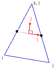
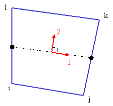
Figure 1: Element Local Results for Linear 2D Elements
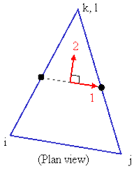
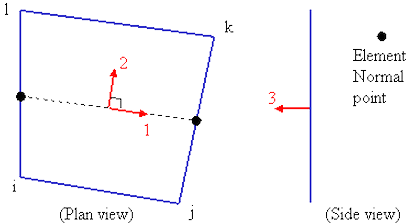
Figure 2: Element Local Results for Linear Membrane Elements
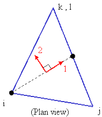
Figure 3: Element Local Results for Linear Plate Elements
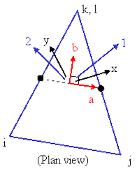
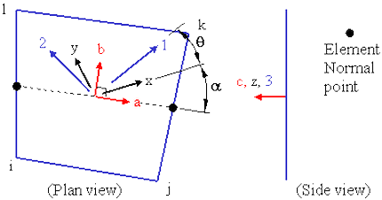
Figure 4: Element Local Results for Linear Composite Elements are in the 1-2-3 direction.
The element local axes (a-b-c) are based on the i-j-k-l sides. The Laminate or Material axes (x-y-z) are rotated α degrees from the element axes (a-b-c). (The material axes are set in the Element Definition on the General tab.) The Lamina axes (1-2-3) are rotated ϑ degrees from the Laminate axes. Axis 1 is parallel to the fibers for each lamina. (The lamina axis is set in the Element Definition on the Laminate tab using the Orientation Angle.)
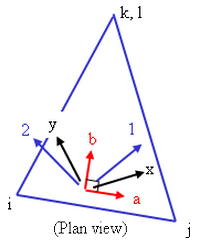
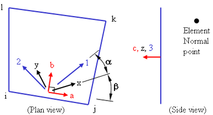
Figure 5: Element Local Results for Nonlinear Elements
2D, Membrane, and Shell (except for Composite) The local 1 axis is parallel to the i-j side.
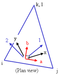
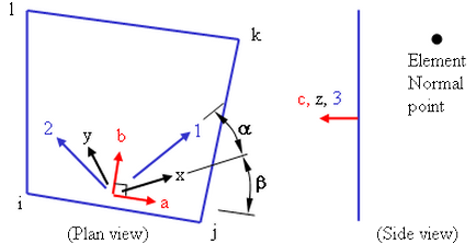
Figure 6: Element Local Results for Nonlinear Composite Elements are in the 1-2-3 direction.
The element local axis a is parallel to the i-j side. The Laminate or Material axes (x-y-z) are rotated b degrees from the element axes (a-b-c). (The material axes are set in the Element Definition on the General tab.) The Lamina axes (1-2-3) are rotated a degrees from the Laminate axes. Axis 1 is parallel to the fibers for each lamina. (The lamina axis is set in the Element Definition on the Composite tab using the Orientation Angle.)
Gaussian Points Results
This command is only available for nonlinear analyses and applies to the element results (stress, strain).
If activated, the result calculated at the Gaussian points are shown in place of the result at the corner node. (Only the Gaussian points closest to the corner nodes are shown.)
Constraint Visibility
This command is only available for structural analyses. Use to quickly verify your model boundary conditions by displaying constraints based on the movement directions or degrees of freedom (DOF) they restrict. If you select exactly the DOF check boxes that correspond to the DOF restricted by a constraint, a triangle displays for the constraint. If you select some of the check boxes that correspond to the DOF restrictions of a constraint, a circle displays for the constraint. If you do not select any check boxes that correspond to a constraint, no symbol displays for the constraint. By default, all check boxes are selected so that constraints which restrict all available DOF display as triangles.
For example, one constraint has the translation in the X and Y directions fixed and another has only the X direction fixed. If you select only the Y Translation check box, the first constraint appears as a circle and the second constraint disappears. If you then also select X Translation, the first constraint displays as a triangle and the second constraint displays as a circle.