Beam elements are two-node members which allow arbitrary orientation in the 3D (three-dimensional) X, Y, Z space. An additional node (K-node) is required to define the element orientation. The beam transmits moments, torque and forces and is a general six (6) degree of freedom (DOF) element (three global translation and rotational components at each end of the member).
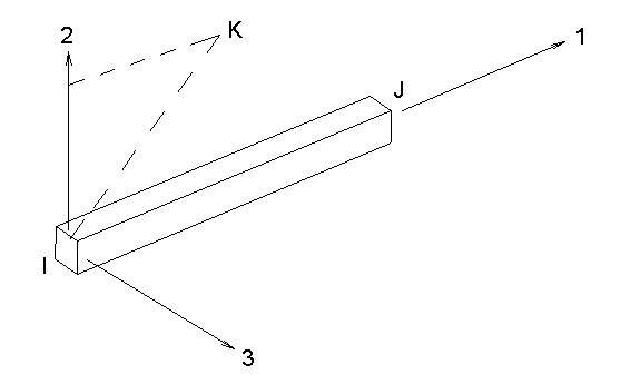
Figure 1: Definition of K-node for Beam Element
The 3D beam element is a three-dimensional uniform cross-section element capable of performing large deformations and elastic-plastic analysis of general beam-frame problems. The cross-section change of shape is not accounted for in any MES/nonlinear structural analysis.
Externally, the beam has six degrees of freedom -- three displacements and three rotations. The output from the analysis includes the end forces of the beam, the axial stress and the associated shear stresses. It supports full 3D translation and rotation motions. The 3D beam element is often used in analyses when bending, torsion and stretching behaviors occur with large deformations and/or material nonlinear effects.
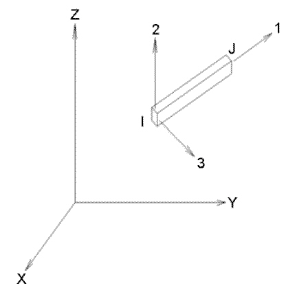
Figure 2: Sample 3D Beam Element
Part, Layer and Surface Properties for Beam Elements
The following chart describes what is controlled by the part, layer and surface properties for beams.
| Part Number | Element data (material model, detailed output, and so on.), stress-free reference temperature, and material properties. |
| Layer Number | Cross-sectional properties (except for General section type). |
| Surface Number | Orientation. |
Beam Element Orientation
Most beams have a strong axis of bending and a weak axis of bending. Since beam members are represented as a line and a line is an object with no inherent orientation of the cross section, there needs to be a method of specifying the orientation of the strong or weak axis in three-dimensional space. This orientation is controlled by the surface number of the line.
More specifically, the surface number of the line creates a point in space, called the K-node. The two ends of the beam element (the I- and J-nodes) and the K-node form a plane (see Figure 3). Beam elements are defined by the local axes 1, 2 and 3, where axis 1 is from the I-node to the J-node, axis 2 lies in the plane formed by the I-, J- and K-nodes, and axis 3 is formed by the right-hand rule. With the element axes set, the cross-sectional properties A, Sa2, Sa3, J1, I2, I3, Z2 and Z3 can be entered appropriately in the Element Definition dialog.
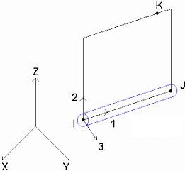
Figure 3: Axis 2 Lies in the Plane of the I-, J- and K-nodes
For example, Figure 4 shows part of two models, each containing a W10x45 I-beam. Note that both members have the same physical orientation. The webs are parallel. However, the analyst chose to set the K-node above the beam element in model A and to the side of the beam element in model B. Even though the cross-sectional properties are the same, the moment of inertia about axis 2 (I2) and the moment of inertia about axis 3 (I3) need to be entered differently.
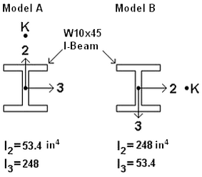
Figure 4: Entering the Cross-Sectional Properties Appropriate for the Beam Orientation
Default K-Node Location (for Beam Orientation by the Surface Number of the Lines)
Table 1 shows where the K-node occurs for various surface numbers. The first choice location is where the K-node is created provided the I-, J- and K-nodes form a plane. If the beam element is colinear with the K-node, then a unique plane cannot be formed. In this case, the second choice location is used for that element.
| Table 1: Correlation of Surface Number and K-Node (Axis 2 Orientation) | ||
|---|---|---|
| Surface Number | First Choice K-node Location | Second Choice K-node Location |
| 1 | 1E14 in +Y | 1E14 in -X |
| 2 | 1E14 in +Z | 1E14 in +Y |
| 3 | 1E14 in +X | 1E14 in +Z |
| 4 | 1E14 in -Y | 1E14 in +X |
| 5 | 1E14 in -Z | 1E14 in -Y |
| 6 | 1E14 in -X | 1E14 in -Z |
Notice that the coordinates of the K-nodes are at an extreme distance from the origin. There is a very good reason for this placement. Consider the limited dimensions of any real-world analysis model. The width, length, and height are insignificant as compared to the distance to the K-node location. For example, if +Z is the upward direction, and you use Surface 2 for the floor joists of a 50 meter wide structure. The deviation of the vertical axis of the beams due to them being displaced +/- 25m (or even 50m) from the Z-axis is infinitesimal. Suppose your length unit is millimeters. The Arc Sin of (50,000mm / 1E14mm) is 0.0000000143° (which is zero for all practical purposes). So, you don't have to define multiple K-nodes for vertically oriented beams even when they are positioned at multiple points across a very wide structure.
You can change the surface number, hence the default orientation of the beams. Select the appropriate beam elements (use the Selection Select Lines command) and right-click in the display area. Choose the Edit Attributes command and change the value in the Surface: field.
User-Defined Beam Element Orientation
In some situations, a global K-node location may not be suitable. In this case, select the beam elements in the FEA Editor environment using the Selection Select Lines command and right-click in the display area. Select the Beam Orientations New command. Type in the X, Y and Z coordinates of the K-node for these beams. To select a specific node in the model, click the vertex, or enter the vertex ID in the ID field. A blue circle will appear at the specified coordinate. Figure 5 shows an example of a beam orientation where you want to define the origin as the k-node.
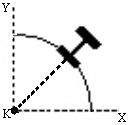
Figure 5: Skewed Beam Orientation
How to Reverse the Direction of Axis 1
The direction of axis 1 can be reversed in the FEA Editor by selecting the elements to change (Selection Select Lines), right-clicking, and choosing Beam Orientations Invert I and J Nodes. This is useful for loads that depend on the I and J nodes and for controlling the direction of axis 3. (Recall that axis 3 is formed from the right-hand rule of axes 1 and 2.) If any of the selected elements have a load that depends on the I/J orientation, you are prompted whether the loads should be reversed or not. Since the I and J nodes are being swapped, choosing Yes to reverse the input for the load will maintain the current graphical display. The I and J nodes are inverted, and the I/J end with the load is also inverted. Choosing No will keep the original input, so an end release for node I will switch to the opposite end of the element since the position of the I node is changed.
How to Verify the Correct Axis Orientation
The orientation of the elements can be displayed in the FEA Editor environment using the View Visibility Object Visibility Element Axis commands. The orientation can also be checked in the Results environment using the Results Options View Element Orientations command. Choose to show the Axis 1, Axis 2, and/or Axis 3 using red, green, and blue arrows, respectively. See Figure 6.
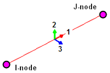
Figure 6: Beam Orientation Symbol
Different arrows are used for each axis.
Specify Cross-Sectional Properties of Beam Elements
There are two options in the Element Definition dialog box that can be used when defining the properties of a beam element. If you are using a common cross-section or one that can be found in one of the pre-installed Beam Cross-Section Libraries, select the Pre-defined option in the Section Type drop-down box and define the properties in the Cross-Section Libraries dialog box. This is done for each layer in the part. Highlight the layer row in the Sectional Properties spreadsheet and click the Cross-Section Libraries button.
- Because nonlinear beams require the actual shape and dimensions of the cross-section, the cross sectional properties (A, J1, I2, and so on.) cannot be entered directly in the spreadsheet. The cross-section library must be used to enter the shape. Likewise, the cross sectional properties (A, J1, I2, and so on) are shown only for reference. The analysis calculates the properties it needs based on the dimensions of the shape.
- See the page Variable Cross-Section Wizard to generate a series of cross-sections along the length of a beam to approximate a tapered beam.
Defining General Beam Properties
If you are using an uncommon cross-section, select the General option in the Section Type drop-down box. The General table will be used to define the cross-section of the beam elements by specifying multiple indices. Each index will be a strip of the cross-section. An index can be a quadrilateral or an arc with a thickness. A quadrilateral index will be defined by two points. These points will be the midpoints of the ends of the quadrilateral as shown in Figure 7(a). An arc index will be defined by three points as shown in Figure 7(b). Points 1 and 3 will be the ends of the arc and Point 2 will be another point on the arc.
|
(a) Quadrilateral section. |
(b) Arc section. |
| Figure 7: Example Strips | |
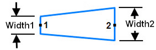

For each strip, define the YY and ZZ coordinates of each point and the width of the segment at that point. The YY coordinate refers to the beam's local 2 axis and the ZZ coordinate refers to the local 3 axis. Both dimensions are measured from the calculated center of gravity of the cross section. he center of gravity of the final shape lies on the beam element's axis. The YY and ZZ coordinates should correspond to the midpoints of the strips.
The Preview window on the Element Definition dialog shows the strips as the data is entered. Note the following features of the Preview window:
- The strip that corresponds to the row with the cursor is highlighted. Move the cursor to a different row of the spreadsheet to view each strip.
- Rotate the mouse wheel to zoom the Preview window in and out.
- Hold and drag the left mouse button to pan the Preview window.
- Right-click and choose Enclose View to see the entire sketch.
Whether a cross section is opened (like an I-beam and channel) or closed (like pipes and tubes) affects the calculation of the torsional constant (J1). These criteria determine how the torsional constant is calculated:
- Closed sections:
- The Section numbers for each index are identical (and not zero).
- The coordinate of the last point on the previous strip matches the first coordinate on the next strip.
- The coordinate of the last point on the last strip in the Section matches the first coordinate of the first strip in the Section. Thus, the strips are continuous within a Section.
- Opened sections:
- The Section numbers for each index are identical (and not zero).
- The strips are not connected together in a closed order.
- Other sections:
- If the Section number is 0, the torsional constant is calculated using the polar moment of inertia (Iyy+Izz). This is true only for round tubes.
Likewise, a general cross-section can consist of multiple subsections. If this is the case, all the indices (rows in the spreadsheet) in each subsection must have the same number in the Section column. If any strips are shared between the subsections, you must specify the Section number of the index that is shared in the Common column. For example, a cross section consists of two subsections, Section 1 and Section 2. Index 2 on Section 1 is identical to Index 5 on Section 2. In the Common column for Index 2, you must enter 2. In the Common column for Index 5, you must enter 1. If a set of indices define a closed cross-section, those indices should be placed in a unique section.
Examples with General Section Type
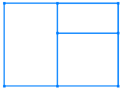
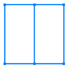
The hollow rectangular cross-section shown in Figure 8(a) would be drawn using four rectangular sections. In order for the software to treat the cross section as a closed cross-section, each point must be used in exactly 2 indices. Therefore the four rectangles shown in Figure 8(b) must be used. It is true that the cross-section geometry will not match the true cross-section perfectly. However, the effect of this difference on the analysis will be small. If you define the four rectangles as shown in Figure 8(c), you will be defining an open cross-section. The effect of using a torsional constant calculated based on an open cross-section for a closed cross-section will be much more significant than a small difference in the other cross sectional values. The cross-section should be defined as shown in Table 2 using the general section type.
|
Theoretical Results: A = 64.0 in2 Iyy = 1301.3 in4 Izz = 1061.33 in4 J1 = 1561.3 in4
(a) Actual Geometry |
Calculated Results: A = 64.0 in2 Iyy = 1281.3 in4 Izz = 1050.3 in4 J1 = 1561.3 in4
(b) Correct Method of Defining the Cross-section. The input for this is shown in Table 2. |
|
Calculated Results: A = 64.0 in2 Iyy = 1301.3 in4 Izz = 1061.3 in4 J1 = 62.2 in4
(c) Incorrect Method of Defining the Cross-section. Since the points between strips do not coincide, the torsional constant calculation will be wrong. |
|
| Figure 8: Hollow Rectangular Cross-Section | |
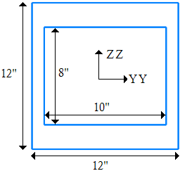
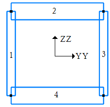
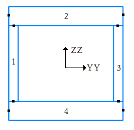
Table 2: Definition of the Cross-Section in Figure 8(b)
| Index | Section | Width (1) | YY(1) | ZZ(1) | Width (2) | YY(2) | ZZ(2) | Common |
|---|---|---|---|---|---|---|---|---|
| 1 | 1 | 1 | -5.5 | -5 | 1 | -5.5 | +5 | 0 |
| 2 | 1 | 2 | -5.5 | +5 | 2 | +5.5 | +5 | 0 |
| 3 | 1 | 1 | +5.5 | +5 | 1 | +5.5 | -5 | 0 |
| 4 | 1 | 2 | +5.5 | -5 | 2 | -5.5 | -5 | 0 |
Four additional cross-sectional geometry types are shown in Figure 9. In all the diagrams, the lines represent a thickness.
|
|
|

|
| (a) | (b) | (c) | (d) |
| Figure 9: Additional Cross-section Geometry Types | |||
Cross-section (a) will require three sections, one for each rectangle. The rectangle on the left will need to be drawn using five indices. The right vertical line must be split into two indices so that they can be defined to be in common with the other two sections. Since common indices must be defined in both sections, this cross-section will require a total of thirteen indices. Cross-section (b) will require two sections. Each rectangle must be defined with the center piece defined as common in both sections. This cross-section will require eight indices. Cross-section (c) will require three sections. Since the two rectangular tube sections are closed sections, they must be defined separately. No indices will be defined as common between any of the sections. This cross-section will require nine indices (it is not necessary to split the sides of the two rectangle where the horizontal piece connects. Cross-section (d) will only require one section. This cross-section will require three indices.
Import General Section Data
The Import button can be used to import the cross-sectional data from a csv file. The csv file must contain 11 columns of data. The values in these columns must correspond from left to right with the column labels in the Coordinates and Dimensions of Section table starting with the Section column. Do not include a column for the Index column.
Cross-Section Libraries
To use the cross-section libraries, the Pre-defined option must be selected in the Section Type drop-down box. Select the layer for which to define the properties in the Sectional Properties spreadsheet, and press the Cross-Section Libraries button.
Use Cross-Sections Libraries
To use the cross-section libraries, first select the layer for which you want to define the cross-sectional properties. After the layer is selected, click the Cross-Section Libraries button.
How to Select a Cross Section from an Existing Library :
- Select the library in the Section database: drop-down menu. Multiple versions of Beam Cross-Section Libraries are provided with the software. (Note: The libraries are set up with I YY (as defined in the AISC manual) corresponding to I 2 in the software.)
- Select the cross section type using the Section type pull-down menu. The type designations available for each of the AISC databases are given in Table 5 of the Beam Cross-Section Libraries page. Additionally, you can use the information in Table 2 of the same page to correlate shape designations from non-AISC libraries with the corresponding AISC section types. This table is not comprehensive because the AISC libraries do not contain all of the cross-section types available in some of the non-AISC libraries.
- Select the cross section name in the Section name: list. You can search for a name by typing a string in the field above the list.
- Review the values in the Cross-sectional properties section of the dialog box. If they are acceptable, click OK.
Create a New Library and Add Cross-Sections to a Library
You cannot modify a pre-installed library in any way. However, you can create custom libraries and add user-defined cross-sections to them. You can also copy a library you make at one computer to a new computer and add it to the program. The procedure for creating custom libraries and cross-sections is outlined on the page Create Custom Cross-Section Libraries and Shape Entries
How to Define Common Shapes
There is a pull-down menu in the upper right corner of the Cross-Section Libraries dialog box that contains a list of common cross-sections that you can specify dimensionally. The included shapes are:
- Round
- Rectangular
- Hollow Rectangular
- Wide-Flange Beam
- C Channel
- L-type (angle)
For all of these shapes, enter the appropriate dimensions. A sketch and data input fields appear after you select the shape.
To select and dimension a common shape
- Go to the Element Definition dialog box for the beam part.
- Ensure that the Section Type is set to Pre-defined.
- Select a layer (row) in the Sectional Properties table and click the Cross-Section Libraries button.
- Choose the User Defined option from the Section database pull-down menu.
- Select the desired common shape from the pull-down menu in the upper-right corner of the dialog box.
- Enter the appropriate dimensions shown at the right side of the dialog box. The cross-sectional properties are calculated and displayed.
- Click OK.
- Repeat steps 3 through 7 for the next layer, or click OK to exit the Element Definition dialog box.
Other Beam Element Parameters
When using beam elements, you must specify the material model for this part in the Material Model drop-down box.
- If the material will remain in the elastic region of the stress-strain curve, select the Isotropic option.
- If the material will experience plastic deformation, select either
- von Mises with Isotropic Hardening. This uses a bilinear curve to control the stress-strain relationship.
- von Mises Curve with Isotropic Hardening. This uses a stress-strain curve with multiple data points beyond the yield stress to control the stress-strain relationship.
- If the material will have different properties based on the temperature but will remain in the elastic region of the stress-strain curve, select the Temperature Dependent Isotropic option. If the material will have different properties based on the temperature but will experience plastic deformation, select the Temperature Dependent Plasticity option.
The Stress Update Method is used when the material model is set to von Mises with Isotropic Hardening. This controls the numerical algorithm for integrating the constitutive equations (stress/strain law) when the material goes plastic. The options available for the Stress Update Method are as follows:
- Explicit: (Original method). This option uses the explicit sub-incremental forward-Euler method for integrating the constitutive equations. The Explicit option is best used for simple problems, such as simple tension, because the method runs faster. However, it is more sensitive to the loading and time step size. The recommended choice for the Nonlinear iterative solution method (set under Setup Model Setup Parameters Advanced Equilibrium tab) is Combined Newton w/ Line Search, depending on the other features in the model which may dictate a different setting.
- Generalized Mid-Point: This option uses an implicit method for integrating the constitutive equations. It reduces the error accumulation and can ensure that the stress updating process is unconditionally stable. Thus, this option is better suited for complicated analyses, such as severe plasticity. The recommended choice for the Nonlinear iterative solution method (set under Setup Model Setup Parameters Advanced Equilibrium tab) is Full Newton 1 w/ Line Search, depending on the other features in the model which may dictate a different setting.
The Parameter for Generalized Mid-point input is used when the Stress Update Method is set to Generalized Mid-Point. Acceptable ranges for this input are 0 to 1, inclusive. When the Parameter is set equal to 0, the resulting algorithm would be a fully explicit member of the algorithm family (similar to the Explicit option for the Stress Update Method); however, the solution is not unconditionally stable. When the Parameter is 0.5 or larger, the method is unconditionally stable. When the Parameter is set to 0.5, the solution is known as a mid-point algorithm; when it is 1, the solution is known as the fully backward Euler or closest point algorithm and is fully implicit. A value of 1 is more accurate than other values, especially for large time steps.
Use the Analysis Type drop-down to set the type of displacement that is expected. Small Displacement is appropriate for parts that experience no motion and only small strains and will ignore nonlinear geometric effects that result from large deformation. (It also sets the Analysis Formulation on the Advanced tab to Material Nonlinear Only.) Large Displacement is appropriate for parts that experience motion and/or large strains. (The Analysis Formulation on the Advanced tab should also be set as required for the analysis.)
 Options Analysis tab and set the Use large displacement as default for nonlinear analyses option to control whether the Analysis Type defaults to small or large displacement.
 If you are using the Temperature Dependent Isotropic or Temperature Dependent Plasticity material model, you must specify a value in the Stress free reference temperature field in the Thermal tab. The thermal stress will be created from the difference between the nodal temperature and this value.
Advanced Beam Element Parameters
Select the formulation method that you want to use for the beam elements in the Analysis Formulation drop-down box in the Advanced tab.
- If the Material Nonlinear Only option is selected, nonlinear material model effects will be accounted for but all calculations will be performed based on the undeformed geometry. Thus, this formulation is suitable for parts with small strains and no motion. This will be the only option available if the Analysis Type on the General tab is set to Small Displacement.
- The Total Lagrangian option will refer to the initial undeformed configuration of the model for all static and kinematic variables. This formulation is suitable for parts with motion and small strains. Note that the material properties should be in terms of engineering stress and strain.
- The Updated Lagrangian will refer to the last calculated configuration of the model for all static and kinematic variables. This formulation is suitable for parts with motion and large strain. Note that the material properties should be in terms of actual stress and strain.
Next select the integration orders for each beam element axis in the 1st Integration Order, 2nd Integration Order, and 3rd Integration Order drop-down boxes. The option in the 1st Integration Order drop-down box will be used for the Gauss quadrature formulation in the primary axis (axis 1, along the length of the element). The option in the 2nd Integration Order drop-down box will be used for the Gauss quadrature formulation in the secondary axis (axis 2). The option in the 3rd Integration Order drop-down box will be used for the Gauss quadrature formulation in the tertiary axis (axis 3). A higher integration order will result in greater accuracy but will lengthen the analysis.
Large rigid body rotation: If any of the elements of the part experience large rigid body rotation at any time period in the analysis, then activate the Large rigid body rotation option. When activated, the rotation matrix is stored at each iteration but leads to more accurate stress results. If the option is not activated and the part experiences rigid body rotation, the stress may increase instead of being constant, leading to some degree of inaccuracy. If the beam elements in the part experience large deformation, then this option does not need to be activated regardless of the rotation (but see the Tip below).
As with any nonlinear, large deflection or large motion analysis, the more steps included in the analysis, the more accurate the results. In some cases, it may be necessary to set the capture rate such that 100 calculation steps occur per 90 degrees rotation of the beam part, or about 1 step per degree of rotation.
Additional Output: There are four types of results output for beam elements that can be created. Whether the additional output is in a text format (read with Notepad, Word, or any text editor) or binary format (read by the Results environment) is indicated below. The formats of the text output files are described in the following page (Beam Element Text Results).
- Detailed force and moment output will output the forces and moments for each beam element at each time step. These results will be written to the summary file (.AL, text format).
- Detailed stress output will output the stress values for each element at each integration point at every time step. These results will be written to the beam stress output file (.BSO, text format).
- Detailed strain output will output the strain values for each element at each integration point at every time step. These results will be written to the beam strain output file (.BST, text format).
- Binary stress and strain output will output the stress and strain values for each element at each integration point at every time step. Since these results are in a binary format, they can be only viewed in the Results environment. If this option is not activated, these results will not be available in the Results environment. Note: The beam stresses shown in the Results environment using the Results Contours Strain Beam and Truss menu are based on the calculated forces and moments divided by the beam cross sectional area and section modulus, respectively. Thus, these results do not take yielding into account. By activating the Detailed stress output or Binary stress and strain output option, the processor will output the calculated stresses - taking all nonlinear effects into account. The Results environment can show the proper stress and strain by using the Results Inquire Inquire Detailed Beam Stress or Results Inquire Inquire Detailed Beam Strain menus if the last option is activated.
Basic Steps for Using Beam Elements
- Be sure that a unit system is defined.
- Be sure that the model is using a nonlinear analysis type.
- Right-click the Element Type heading for the part that you want to be beam elements.
- Select the Beam command.
- Right-click the Element Definition heading.
- Select the Edit Element Definition command.
- In the General tab, select the appropriate material model for this part in the Material Model drop-down box and the shape of the cross-section in the Section Type drop-down box.
- If you selected the Pre-defined option in the Section Type drop-down box, select the Layer to define in the Sectional Properties spreadsheet and press the Cross-Section Libraries button. Select or enter the cross-section.
- Alternatively, if you selected the General option, define the cross-section in the table that will appear.
(See the Specify Cross-Sectional Properties of Beam Elements topic above.)
- Press the OK button.