Some of the commands for the Thermal Result are identical to the Linear Results. Below are the commands that are unique to thermal analyses.
Calculated Temperature
(units: degrees) This is the resultant temperature for the currently shown time step (transient analyses) or load case (steady state analyses).
Initial Temperature
(units: degrees) Shows the temperature at time 0. This value does not change with different time steps or load cases. For steady state analyses, this temperature is used to estimate the material properties for temperature-dependent materials.
The Initial Temperature shows temperatures read from another thermal model, the default nodal temperature, or "Initial Temperature" manually applied to the model in the FEA Editor. Initial Temperature does not show the applied loads, such as Controlled Temperature or convection ambient temperature.
Heat Flux
(units: energy/length^2/time) If active, the display will be based on the flux magnitude, or the specified global direction, at the element centroid. The heat flux at the centroid is calculated using Fourier's law and the temperatures at the nodes.
Heat Rate Through Face
(units: energy/time) If active, the display will be based on the heat rate normal to the associated face. A positive value indicates the heat is flowing out of the element through the face; negative indicates the heat is flowing into the element through the face.
The calculated value for the heat flux at the centroid (hfcg) is used to calculate the heat rate of the face (H) as follows:
H = (component of hfcg normal to the face)*(Area of face).
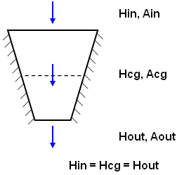
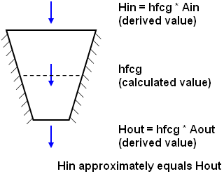
This can lead to some apparent discrepancies when the elements are skewed or the faces of the elements are not parallel and perpendicular to the heat flux vector. For example, imagine a steady state situation of heat flowing through one trapezoidal element with insulated sides (see Figure 1(a)). In reality, the heat flowing in (Hin) equals the heat out (Hout). In the FEA process, the heat flux at the centroid is calculated (hfcg), and then the heat flow through the faces is derived. As shown in Figure 1(b), this leads to an approximation which results in the two heat rates with slightly different values.
|
|
| (a) In a hypothetical model, the heat rate (H) passing through any area is equal, whether at the inlet face, the centroid (cg), or the outlet. | (b) In FEA, the heat flux (hfcg) calculated for the centroid is used to calculate the heat rates (H) through the faces. If Ain and Aout do not equal Acg, the heat in will not equal the heat out. |
|
Figure 1: Heat Rate Through Face Calculation H = heat rate, A = area, hf = heat flux |
|
This calculation procedure can also result in situations where the heat rate through face shows a small heat value going through an adiabatic wall (see Figure 2), or similar to Figure 1, a situation in which the heat leaving the boundary of one part does not equal the heat entering another part (see Figure 3). These effects are due to the approximation of the heat rate calculation.
Hout = hf n * Area of face
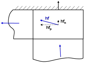
Figure 2: Heat Rate through Face Projected From Heat Flux
For the heat rate passing through a face, the heat flux vector (hf) is broken into components parallel (hfp) and normal (hfn) to the face. The small normal component can appear to violate the adiabatic condition. A smaller mesh at the wall can help minimize such problems. Alternatively, add a small, insignificant convection load to the adiabatic face and set the Heat Flow Calculation drop-down on the Element Definition dialog to Linear Based on BC.
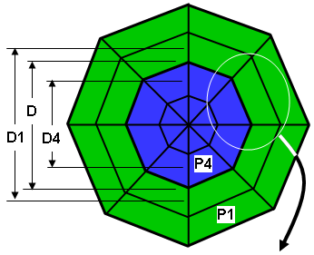 |
(a) A two part model: part 1 (green) on the outside and part 4 (blue) on the inside. The diameter of the centroid of the inner elements in part 1 is D1. The diameter of the centroid of the outer elements in part 4 is D4. |
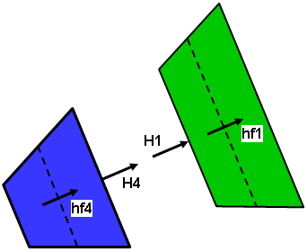 |
(b) Detail of two elements from the model, shown magnified and separated for clarity. The heat fluxes hf4 and hf1 are calculated from the temperature distribution. The heat rate leaving the outer face of part 4 (blue) is proportional to H4 ~ hf4 * D. The heat rate entering the inner face of part 1 (green) is proportional to H1 ~ hf1 * D. Since the diameter D is slightly different than the diameters of the centroids D1 and D4 where the heat flux is calculated, the two heat rates will not be identical. |
| Figure 3: Heat Rate Through Face Example | |
For interior faces, the heat flowing out of one element and into an adjacent element should be equal (and opposite in sign). Therefore, the smoothed value should be zero. To see the magnitude of the heat flow in this situation, deactivate the Results Contours  Settings Smooth Results.
To sum the heat flow through a set of faces, use the Results Inquire Inquire Current Results. Select the faces (Selection Select Faces) and then change the Summary drop-down box to Sum.
- Since surfaces can also be selected to get the heat flow rate result, it is convenient if the faces are placed on a unique surface when the model is being built. Then this surface can be selected (Selection Select Surfaces) in the Results environment and Results Inquire Inquire Current Results can be used to sum the values.
- If the faces being summed have an applied load, such as a convection or radiation, then consider using the Filter Modules in the browser to make selecting the faces easier. (See the Browser Functions page.)
- The Heat Rate Through Face for a 2D axisymmetric analysis gives the total heat flow for a full revolution (360 degrees = 2*pi).
For brick elements, the outside faces are displayed. To view the inner faces, you should use the Results Options View Shrink Elements to look between each element and then Results Options View Show Internal Mesh to display the interior faces.
Heat Flux Precision
Precision is a method of highlighting stepped changes in results from one element to the next. In an ideal model, the heat flux would change smoothly between adjacent element. In the process of discretizing the model with elements, there will always be some change in results from one element to the next. The results are not continuous.
In thermal analyses, the precision is based on the discontinuous heat flux magnitude from element to element (across element boundaries). It is calculated as follows:
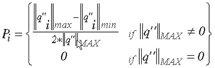
where:
P i is the precision at node i,
![]() max is the maximum heat flux magnitude at node i obtained by finding the maximum over its neighboring elements,
max is the maximum heat flux magnitude at node i obtained by finding the maximum over its neighboring elements,
![]() min is the minimum heat flux magnitude at node i obtained by finding the minimum over its neighboring elements,
min is the minimum heat flux magnitude at node i obtained by finding the minimum over its neighboring elements,
![]() MAX is the global maximum of the heat flux magnitude.
MAX is the global maximum of the heat flux magnitude.
Based on the formula, the range of precision values is 0 to 0.5, inclusive.
If the model is partially hidden, the precision calculations are based on the restricted set of nodes and elements. Nodes which belong to a single element will have a precision of zero.
Liquid Fraction
When any of the parts of a transient heat transfer analysis are set to a phase change material model, the Liquid Fraction will appear in the Results Contours Heat Flow Phase Change. A value of 1 indicates the node is liquid, a value of 0 indicates the node is solid, and values in between indicate a state of melting or freezing and what fraction of the mass is liquid. Nodes which belong to parts that are not set to a phase change material model will not be shaded with the result.