Each of the display options discussed on this page are found in one of the following locations:
- Context Menus (accessed by right-clicking with parts, surfaces, or elements selected)
-
Ribbon Tab
 Panel :
-
Results Contours Settings
-
Results Options View
-
Results Options View Settings
-
Results Options Other
-
Results Contours
Commands Found in the Context Menu for Selected Parts, Surfaces, or Elements
Visibility
Click Visibility to hide the selected parts, surfaces, or elements.
Isolate
Click Isolate to hide all of the unselected parts, surfaces, or elements, leaving only the selected ones visible.
Show All
Click Show All to restore the visibility of all hidden parts, surfaces, and elements. This command appears in the context menu whether entities are currently selected or not.
Commands found under Results Contours Settings
Save to Default Settings
If this command is selected, the current display settings will be saved as the defaults for all future models. This includes, result contour settings, legend box settings, annotations, and curve settings.
Reset to Default Settings
If this command is selected, the default settings will be loaded and applied to the model. The default settings can be saved using the Save to Default Settings command.
No Contour on Kinematic Elements
If this command is active, any parts of 2D or 3D kinematic elements will be displayed by part color instead of the results contour. If this option is not active, these parts will be displayed with the results contour if it is applicable (stress is not an applicable result for kinematic elements). If the results contour is not applicable, the part will be displayed as a wireframe. This command will only be available for a nonlinear analysis.
Results found under Results Options View
Element Visibility Hide Selected Elements
Any elements that are currently selected when this command is activated will disappear from view. They can be viewed again by executing the Show All command.
Element Visibility Hide Unselected Elements
Any elements that are not currently selected when this command is activated will disappear from view. They can be viewed again by executing the Show All command.
Element Visibility Show All
All elements will return to view (visible and available for selection) after this command is selected. None of the elements are hidden.
For solid meshes (bricks, tetrahedra, and so on), elements that are not hidden may still be invisible and may not contribute to the results shown in the display and legend. Refer to the Show Internal Mesh section on this page for an explanation.
Mitre Visualized Beams
If this command is selected, a mitre operation will be performed where beam elements meet at an angle. This will show a more realistic representation of the 3D geometry. If the mitre operation results in inaccurate geometry, verify that the i and j coordinates are consistent along the length of the beam.
Show Internal Mesh
This command only effects models with solid elements (bricks, tetrahedrons, and so on).
By default, only the surface mesh of a solid part is shown. If this command is activated, the entire solid mesh will be displayed for elements that are not hidden. (Results Options View Element Visibility Show All is used to display hidden elements.)
When displaying a result, this option also affects the values shown in the legend and the maximum and minimum probes. When displaying only the surface mesh (Show Complete Mesh is not activated), the range shown in the legend is based only on the nodes on the elements attached to the surface. If the complete mesh is shown (Show Complete Mesh activated), then the range in the legend and probes are based on the complete mesh: the inside mesh and surface.
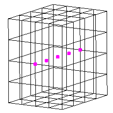
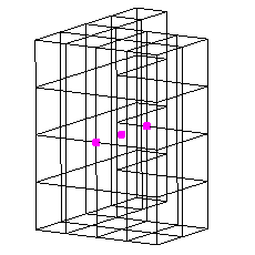
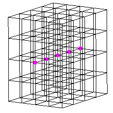
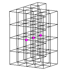
Whether the complete mesh is activated of deactivated, elements and nodes on the interior can still be selected, either with the mouse or by specifying the appropriate number under Results Inquire Inquire Element Information Specify. See Figure 1 below.
| Show All activated (default): | Some elements hidden: | |
|---|---|---|
| Show Complete Mesh deactivated (default) |
All nodes and elements are available for selection, but the interior mesh is not shown. |
Nodes on the hidden elements cannot be selected. The interior mesh is not shown. |
| Show Complete Mesh activated |
All nodes and elements are available for selection, and the interior mesh is shown. |
Nodes on the hidden elements cannot be selected. The interior mesh is shown. |
|
Figure 1: Show Complete Mesh Behavior with and without Hidden Elements The unshaded mesh is shown to reveal the details of the inside. In each figure, a selection rectangle was used to select the nodes through the thickness, as indicated by the magenta selection dots. |
||
Show Wireframe During Movement
System resources are used when the model is dynamically rotated, zoomed, or panned – (using the mouse or the commands View Navigate Orbit, View Navigate Zoom Zoom, and View Navigate Pan, respectively). The speed at which the model responds to the movement of the mouse can be improved by activating the Show Wireframe During Movement option. When activated, the model is shown without any shading while the viewpoint is dynamically moving. When not activated, the shaded model is displayed while the viewpoint is moving.
Shrink Elements
This command will allow you to shrink all the elements about their centroid. A slider bar appear so you can shrink them to the appropriate factor.
Show Numbers Node Numbers
This command will cause the node numbers to be displayed on the model. These numbers are generated during the decoding process.
Show Numbers Element Numbers
This command will cause the element numbers to be displayed on the model. These numbers are generated during the decoding process.
Element Orientation
This command will allow you to show the orientation information for the relevant element types.
Use the Element Orientations commands to display the element 1, 2, or 3 axis directions with a red, green, or blue arrow, respectively. Plate, 2D, membrane, and beam elements have local orientations. The 1-2-3 direction is important to know for a variety of reasons, such as when viewing the stress tensor results in local element coordinates (see Results Contours Settings Use Element-Local Results), or for beam stresses about the local axes, or for a temperature difference through the thickness of a plate element. Each axis arrow points in the positive direction. For composite elements, the Element Orientations show the element's a, b, or c axis directions.
If you select the Material Axis Orientation command, an arrow will appear pointing in the direction of the principal material axis for each element. The principal material axis is defined as follows:
| Material Model or Element Type | Principal Material Axis |
|---|---|
| Isotropic | Same as local element axis 1 |
| Orthotropic (except for composite elements) | Points in direction of modulus of elasticity E1 |
| Composite elements | Points in direction of Laminate (material) axis x. The angle of the fibers for each lamina (q) are measured from the Laminate axis x. |
 Options Results Global FEA Objects Preferences.
 Commands found under Results Options View Settings
Lighting
If you do not want the model to be shaded using a light source, you can deactivate this option. The model will now be colored according to the part number or the results contour with no effects of lighting.
Background Image
This command will allow you to select an image file to display in the background of the display area. You will also be able to have this image appear in any images that you save.
Transparency Level
When this command is executed, a Transparency dialog will appear. The sliders will allow you to control the transparency level of the following items:
- Model: The transparency of all the parts and surfaces that are currently transparent can be adjusted. (Activate the transparency of parts and surfaces by selecting the relevant entry in the tree view, right-click, and choose Draw Transparently.)
- Slice Planes: The transparency of all slice planes can be adjusted. (Slice planes can be shown or hidden by selecting the relevant slice plane in the tree view, right-click, and choosing Show or Hide.)
- Impact Planes: The transparency of all impact planes can be adjusted. (Impact planes can be shown or hidden by using Results Options View Settings Impact Plane Visibility.)
Minimum Break Angle for Features
Use this command to set the angle that will be used to define the feature lines of a model. If the normals of any two adjacent faces intersect at an angle greater than this value, a feature line will be defined.
Slice Planes
Use the available slice plane commands to create, activate, deactivate, or manipulate the visibility, position, and orientation of slice planes. In order slice plane editing commands to be active, you must have an active slice plane in the current presentation window.
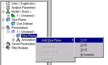
You can use the ribbon commands or a context menu to create a slice plane. For the latter method, right-click the Slice Planes heading in the Presentation section of the browser, as shown in the image below. Select the Add Slice Plane command and then select one of the options in the next pull-out menu.
Once one of the four slice plane options is selected, it will appear on the model and the commands under Slice Planes in the ribbon will become active.
If another slice plane is created while a previously created one is still in Edit mode, the same editing option remains active for the new slice plane. However, if Edit mode is canceled, then the default editing option (Translate Parallel) is restored the next time you edit any slice plane.
To return to Edit mode, you must right-click a previously defined slice plane heading under the current Presentation in the browser and choose Edit (as shown in the following image):
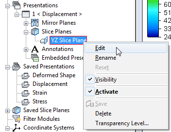
The remaining commands in the Slice Plane context menu of the browser are as follows:
- Rename: Specify a user-defined name for the slice plane. This command is especially useful if you plan on saving your slice plane as a User-Defined one (available for future models).
- Reset: This command is only available while in Edit mode. Click Reset to undo the current changes, restoring the slice plane orientation to what it was when you entered Edit mode.
- Visibility: This command toggles the visibility of the slice plane itself. The model remains sliced in either case. Only the visibility of the plane and the I and J axis lines is affected.
- Activate: This command toggles the active state of the slice plane. When on, the sliced portion of the model is hidden. When off, the model is displayed normally.
- Save: This command is only available while in Edit mode. Click Save to save the current slice plane to the User Defined list under the Saved Slice Planes heading in the browser. Saved slice planes are available for use in future models. Simply right-click a user-defined slice plane heading and choose the Add To Active Presentation command.
- Delete: This command deactivates and removes the current slice plane from the presentation.
- Transparency Level: Access the Transparency dialog box to control the transparency level of the model and slice plane. Move the sliders towards the right for more opacity and towards the left for more transparency.
Use the subcommands under Slice Planes in the ribbon (Results Options View Settings Slice Planes) to choose the desired Edit mode (see below).
Slice Plane Commands:
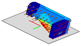
A sample slice plane is shown below. The descriptions of the slice plane commands refer to this image.
Access the following editing commands from the ribbon (Results Options View Settings Slice Planes)
- Change the Location or Orientation of a Slice Plane (Edit Mode):
- The Rotate About I command rotates the plane about the local i axis. This is the red axis on the slice plane.
- The Rotate About J command rotates the plane about the local j axis. This is the green axis on the slice plane.
- The Rotate About Origin command rotates the plane about the origin of the slice plane. The origin is at the intersection of the i and j axes. When one of these commands is selected, you can rotate the slice plane by clicking the left mouse button and dragging the mouse across the screen. The slice plane will rotate to follow the mouse.
- The Translate Parallel command moves the slice plane along the axis normal to it, keeping it parallel to the starting orientation. This translation is done by clicking the left mouse button and dragging the mouse across the screen. The slice plane translates to follow the mouse. Translate Parallel is the default editing option when a new slice plane is created and whenever you return to the Edit mode.
- Change the Side of the Slice Plane on which the Model is Visible (Edit Mode): By default, the slice plane will show the portion of the model on the positive side of the plane. The positive side of the plane is determined by the cross product of the i and j axes.
When you click the Flip command, the portion of the model on the positive side of the plane will be hidden and the portion on the negative side will appear. Click it again to return to the originally displayed side.
- Saving Slice Planes (Edit Mode):
The Save command saves the current orientation and location of the plane as a user-defined plane. After this command is clicked, the plane will be located in the User-Defined section under the Slice Planes heading in the browser. These slice planes will be available for any future models.
-
Sliced model display option: Use transparency instead of invisibility.
The Draw Sliced Elements Transparently option renders the portion of the model on the hidden side of the slice plane transparently instead of making it invisible. This viewing option enables you to see into the interior of a part or assembly while still maintaining visibility of the entire model.
Impact Plane Visibility
This command will access the Impact Planes Settings screen. Each impact plane in the model will be listed in this screen with a check box. Deactivating a check box will cause that impact plane to disappear from the display area.
Import Presentations (Results Options Other Tools Import Presentations)
If you have saved a presentation in a previous model, you can import those saved settings using this command. This will access a File Open dialog where you can select the necessary *.FEM file for the previous model. All saved presentations from all design scenarios in the selected file will be imported.
The imported presentation can be applied to the current model by double-clicking on the entry, or by right-clicking and choosing Activate.