The maximum temperature at 1200 seconds is slightly more than 100°F. Next, we graph the temperature versus time of the hottest node.
- Click
 Results Inquire
 Probes Maximum to locate the hottest node.
 - With the
 Selection Shape Point or Rectangle and
  Selection Select Nodes commands active, click the node to which the maximum temperature probe is pointing. This node is near the middle of the top surface of the processor chip, as shown in the following image:
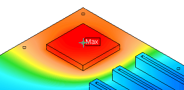
- Right-click in the display area and select Graph Value(s). A graph displays, which looks like the following image:
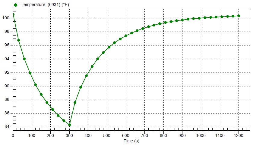
The temperature of the selected node decreases about 26°F during the first 300 seconds (the cool off period). The temperature is still about 4° warmer than the ambient temperature at 300 seconds. Heat generation resumes at the rate of 5 Watts at 301 seconds and continues at that level for the remainder of the simulation event. During this 15 minute period, the chip almost reaches the steady-state temperature again (within 0.5°F).
Notice the nonlinear cooling and heating rates:
-
The cooling rate (slope of the temperature versus time curve) decreases as the ambient temperature is approached. The rate of convective heat loss is proportional to the difference between the surface and ambient temperatures. So, when the surface temperature is close to the ambient temperature, the convective heat loss approaches zero.
- The heating rate slows as the convective heat loss magnitude approaches equilibrium with the heat generation magnitude. When the processor is re-energized, the temperature initially increases quickly because heat input (generation) is relatively high while convective heat loss is relatively low.
-
This tutorial is now complete.