Thermal analysis
In the 05 directory, use a text editor to create the files named fin.in and fin_path.lsr with the contents shown in "Local Simulation Input Files" for Example 5. Run the analysis from the command line:
$ pan -b fin
After the analysis completes, the last few lines of the output file fin.out should be similar to the following:
inc =      4100 time =   500.00000     iter =    1 eps =   0.47875E+01
inc =      4100 time =   500.00000     iter =    2 eps =   0.14060E+01
inc =      4100 time =   500.00000     iter =    3 eps =   0.73374E-01
inc =      4100 time =   500.00000     iter =    4 eps =   0.20848E-03
Increment end
Analysis completed
CPU wall=  223.3203    CPU total=  4454.921
END PROJECT PAN
Mechanical analysis
In the 05 directory, use a text editor to create the file named fin_mech.in with the contents shown in "Local Simulation Input Files" for Example 5. Run the analysis from the command line:
$ pan -b fin_mech
After the analysis completes, the last few lines of the output file fin_mech.out should be similar to the following:
inc = 4167 time = 500.00000 iter = 1 eps = 0.81453E+04
inc = 4167 time = 500.00000 iter = 2 eps = 0.48872E+04
inc = 4167 time = 500.00000 iter = 3 eps = 0.31306E-09
Increment end
Analysis completed
CPU wall= 433.6602 CPU total= 8417.543
END PROJECT PAN
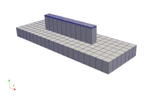
Figure 5.2: LENS part discretized by 8-node linear hexahedral elements. Dummy boundary conditions, materials, and properties must also be applied.
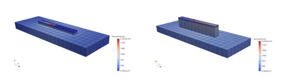
Figure 5.3: Temperature results (oC) during the deposition of the final layer.
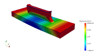
Figure 5.4: Post-process z distortion (5x magnification)
The results can be viewed in ParaView by importing the CASE files.