To solve flow in networks, numerically, the network must be represented, algebraically, on the computational domain.
The Coolant Flow solution scheme is a node method, based on the well-known SIMPLE algorithm of Patankar and Spalding. Given a series of parallel channels, as shown in figure 1, with three branches, 1, 2, and 3 that diverge at junction A, and reconverge at junction B, this flow network must be broken down into nodes and elements for computational purposes.
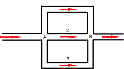
Figure 1. Parallel flow through a network
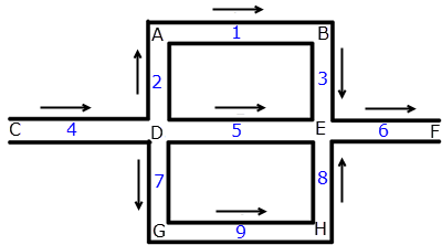
Figure 2. Computational domain of the parallel flow network
In figure 2, using the same series of parallel channels as shown in figure 1, nodes are represented by letters, and elements by numbers. Each element joins two nodes. Consider node D, which has 4 branches associated with it. Node D is connected to nodes A, C, E, and G by elements 2, 4, 5, and 7. Algebraically, this can be expressed as node i is connected through elements eij to neighbouring nodes nij , where j is the number of branches associated with node i .
Connectivity arrows show the orientation of the element. Every node in the network has a connectivity operator associated with each of its branches, that determine the direction of flow in the branch. When the connectivity arrow points towards the node, the connectivity operator is (+) for the adjoining node. So for node D, where only 1 connectivity operator points towards it, the only positive connectivity operator is for node C. The other three connectivity operators are all (-).
The continuity equation and the temperature equation both need to be satisfied on every node in the network. The work-energy principle equation needs to represent the pressure drop relationship on every element in the network.