Section 19: Flexural Test Fixture Exercise

Introduction

In this exercise, we will duplicate the three-point bending test required in ASTM D638 for plastic material flexural testing. Our analysis will feature a section of polymer (acrylonitrile butadiene styrene) subjected to a uniform stress (uniaxial tension test) in a test rig. We will setup a nonlinear material model, and will intentionally over-deform the beam into the apparent nonlinear and post-yield range of the material. Finally we will unload the test bar to look for permanent deformation.

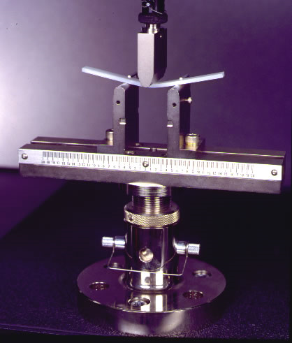
It is important to note that some polymers behave differently in tension and compression. In such materials, the Flexural Modulus = Average Modulus. Nonlinearities cause stress redistribution during bending, meaning that linear calculations are no longer valid.

To reduce simulation time, we will use quarter symmetry of the model.

1. Open the Model and Start the Autodesk Inventor Nastran Environment

Start Autodesk Inventor, and open Flex Test.iam from the Section 19 - Flex Test Fixture sub-folder of your training exercises folder. (Get Started > Launch > Open)

From the ribbon, click the Environments tab, and click Autodesk Inventor Nastran.

You should see this:

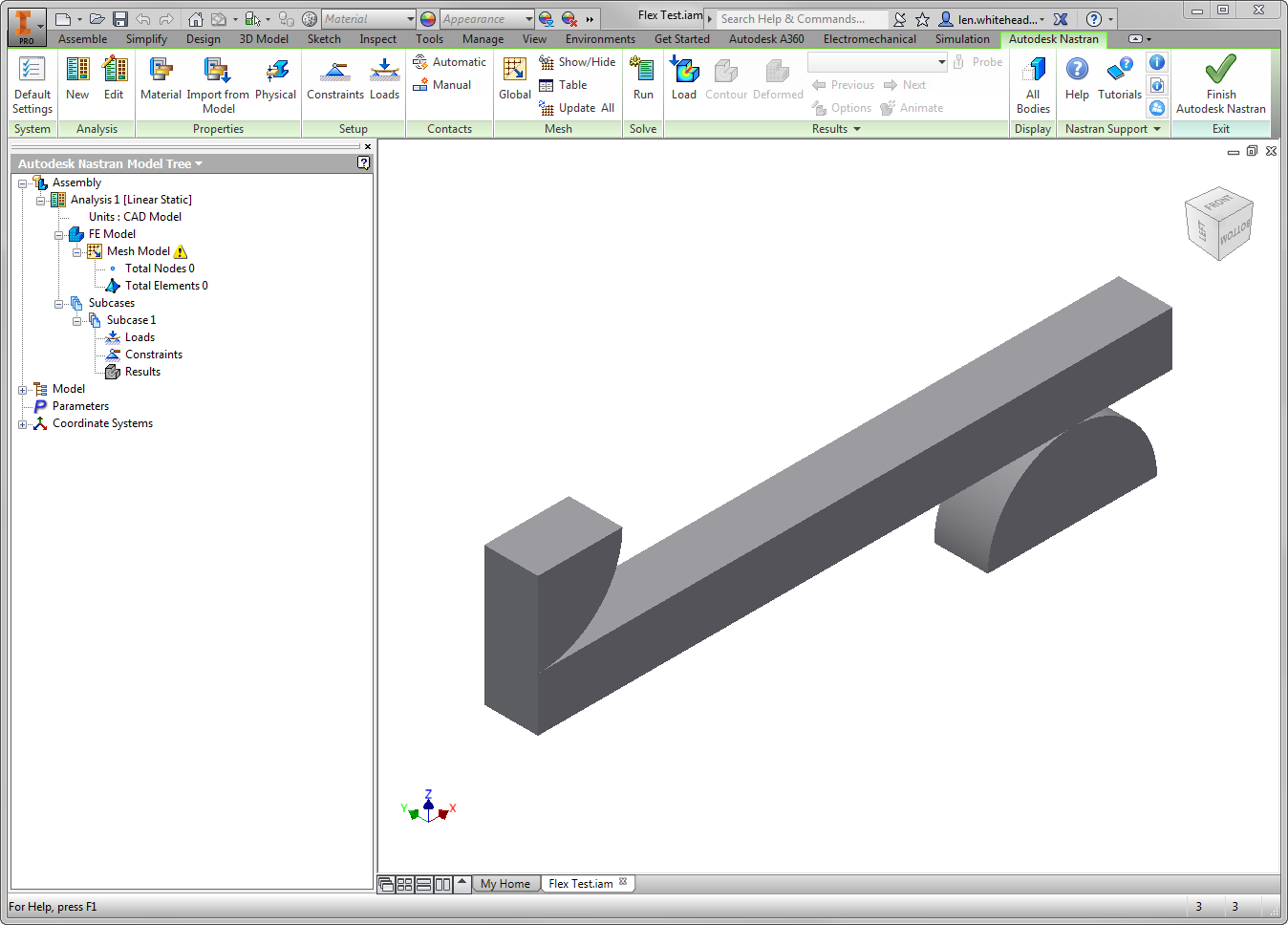
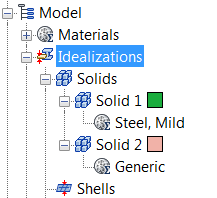
In the Model tree, expand Idealizations. If any Idealizations are already defined, like Solids 1 and 2 below, right-click Idealizations > Delete All, to ensure that no unwanted materials can participate in the analysis.

2. Change the Analysis Type

1. From the Analysis tree, right-click Analysis 1 > Edit.
2. On the Analysis dialog, set the Type to Nonlinear Static.
3. On the Options tab, verify that Large Displacements is On.
4. On the Output Controls tab, Output Sets group, make sure that Stress and Strain are checked.
5. Click OK.

Because stress-strain curves for plastic materials often have shallow slopes in the plastic region, it is preferable to view results in terms of strain.

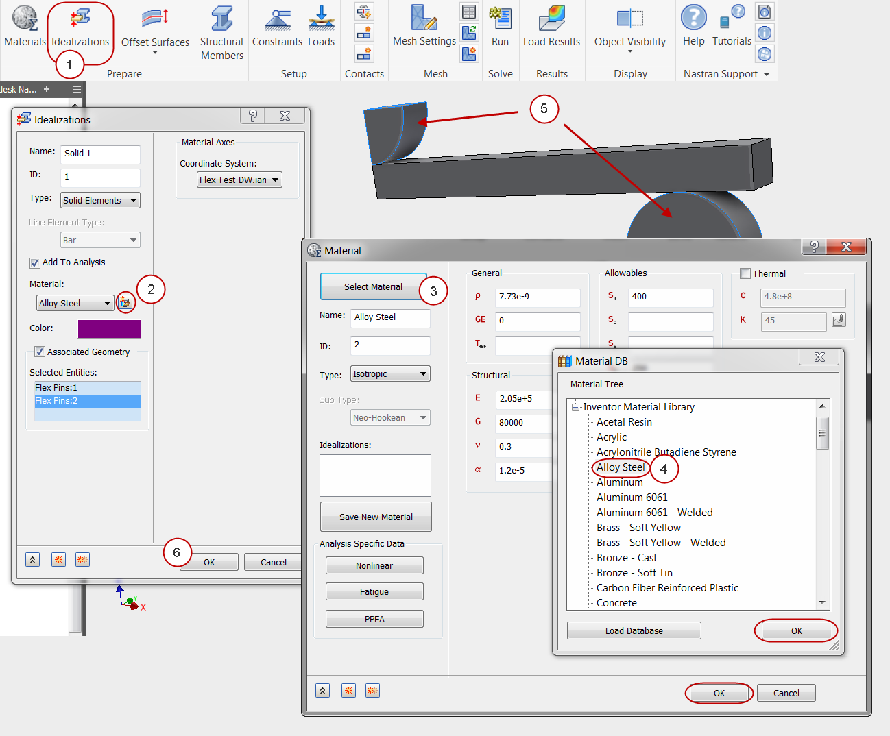
3. Assign the Alloy Steel Property

1. Click Idealizations from the ribbon.
2. Click the New Material icon.
3. On the Material dialog, click Select Material. Expand the Inventor Material Library, and select Alloy Steel. Click OK and OK to close the two Material dialogs.
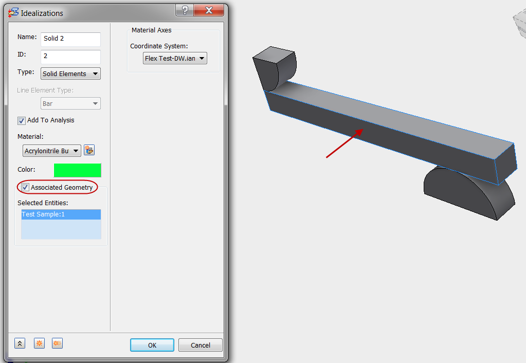
4. In the Idealizations dialog, check the Associated Geometry box.
5. Select the load pin and the support parts.
6. Click OK.

4. Assign and Define the Nonlinear ABS Material

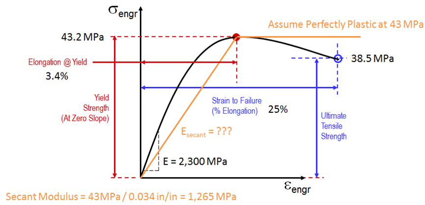
The typical ABS stress-strain curve (from Matweb Averages) looks like this:

1. Click Idealizations from the ribbon.
2. Click the New Material icon.
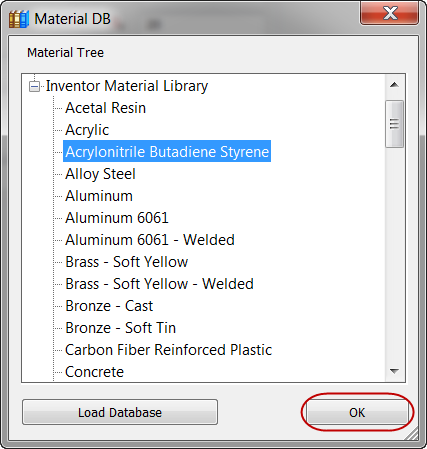
3. On the Material dialog, click Select Material. Expand the Inventor Material Library, and select Acrylonitrile Butadiene Styrene. Click OK.



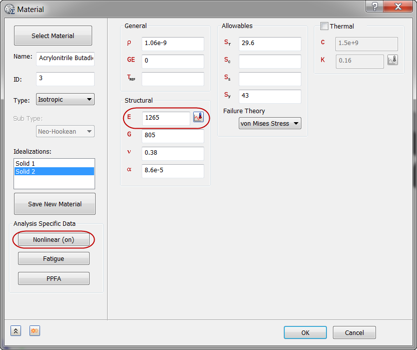
4. In the Material dialog, set the value of E to 1265 MPa.
5. Click Nonlinear.



6. On the Nonlinear Material Data dialog, set the Type to Plastic.
7. Make sure the Hardening Rule is set to Isotropic.
8. Set the Initial Yield Stress to 43 MPa.
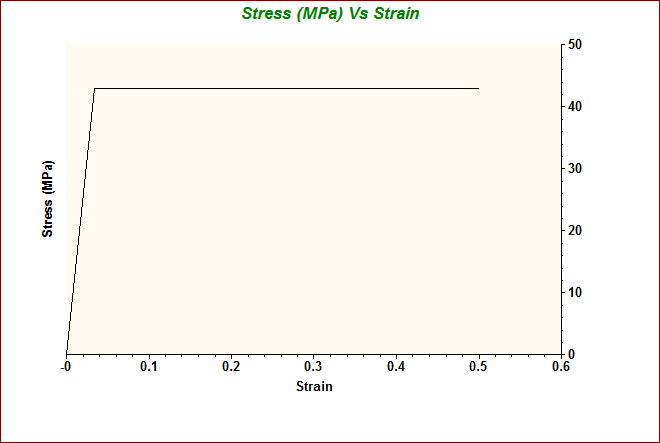
9. In the table, double-click in the Strain column in the first open row, and enter 0.5. (This is 50%.)
10. Click in the adjacent Stress cell, and enter 43.
11. Click Show XY Plot.





12. Click OK twice.
13. Check the Associated Geometry box.
14. Select the test part.
15. Click OK.

5. Apply the Y Symmetry Constraint

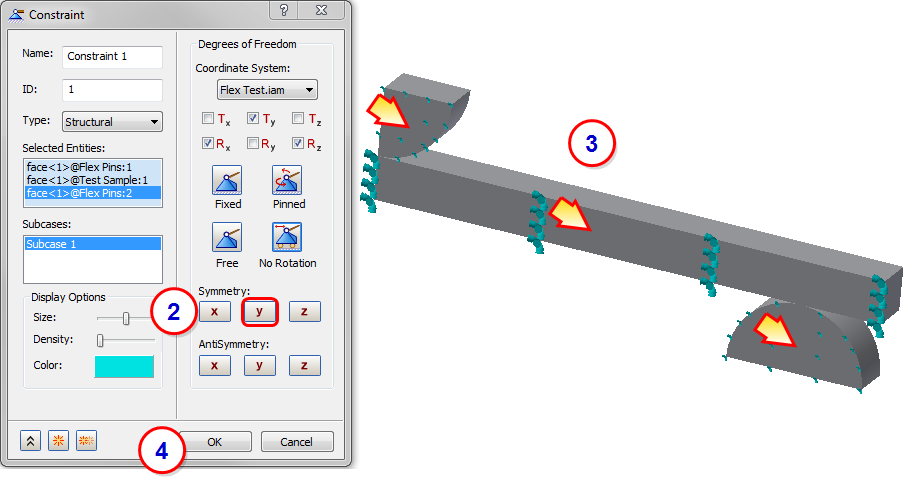
1. Click Constraints from the ribbon.
2. Click Y Symmetry.
3. Click the faces shown.
4. Click OK.

6. Apply the X Symmetry Constraint

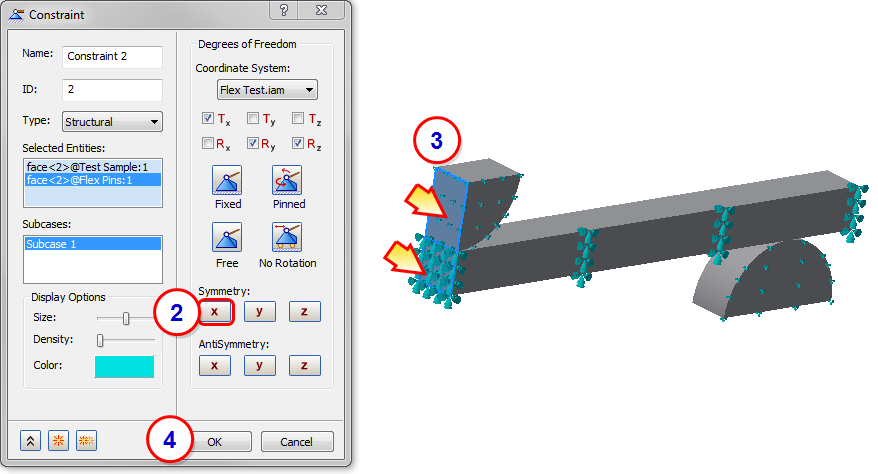
1. Click Constraints from the ribbon.
2. Click X Symmetry.
3. Click the faces shown.
4. Click OK.

7. Apply the Fix Constraint to the Support Pin

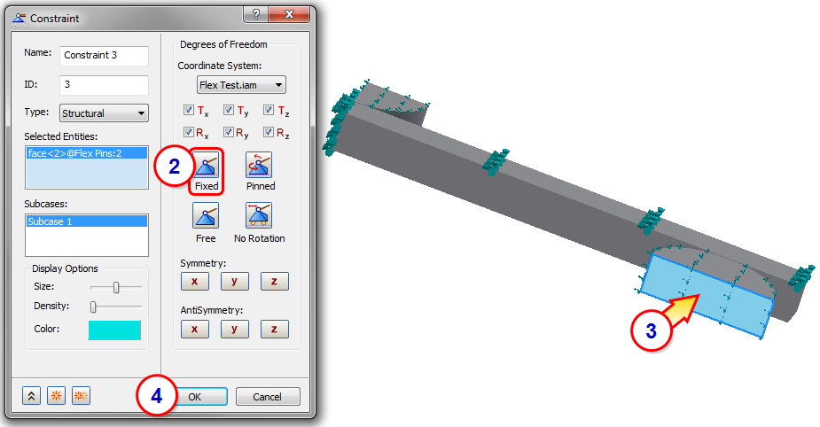
1. Click Constraints from the ribbon.
2. Click Fixed.
3. Click the face shown.
4. Click OK.

8. Apply a Pushing Constraint

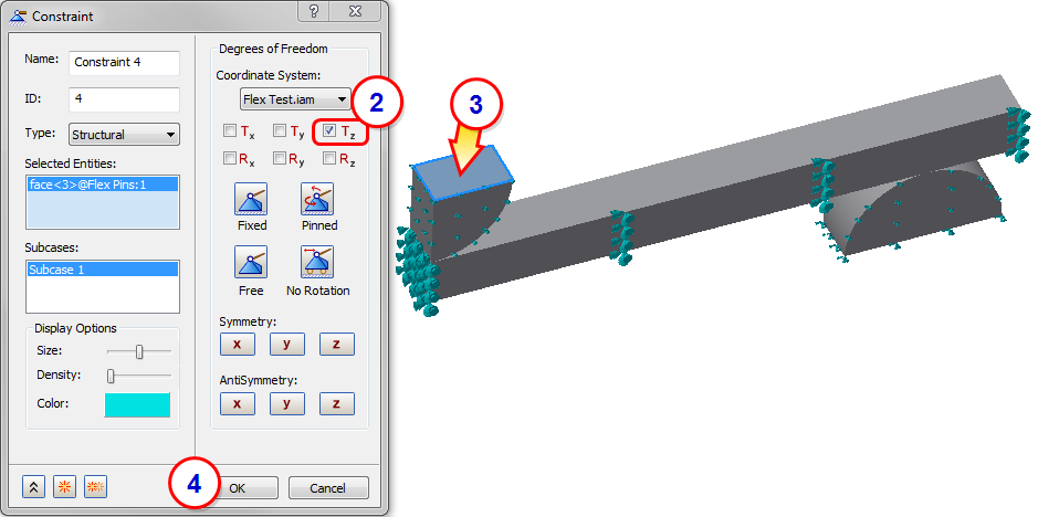
The pin loading will push the center of the beam through a defined displacement. This enforced displacement is defined as a combination of this constraint and a pushing load that we will define in the next step.

1. Click Constraints from the ribbon.
2. Make sure all degrees of freedom are unchecked except for Tz.
3. Click the face shown.
4. Click OK.

9. Apply the Pushing Load

1. Click Loads from the ribbon.
2. Set the Type to Enforced Motion.
3. Set the Sub Type to Displacement.
4. Set the Tz value to -3.
5. Select the face shown.
6. Click OK.

10. Define Contacts

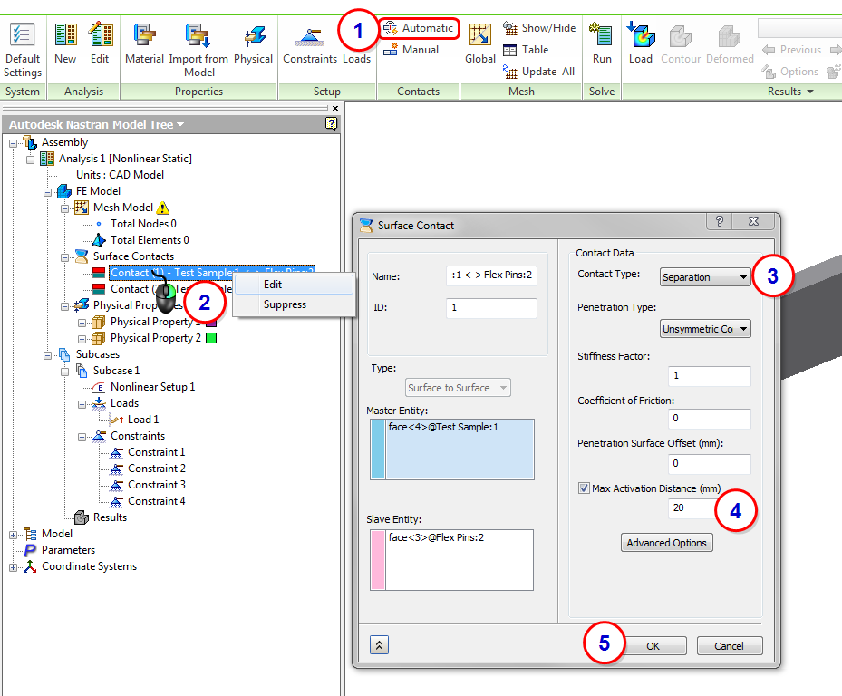
1. Click Automatic from the Contacts panel in the ribbon.
2. From the Analysis tree, expand the Surface Contacts branch, right-click on the first contact, and click Edit.
3. Change the Contact Type to Separation.
4. Specify 20 as the Max Activation Distance.
5. Click OK.
6. Repeat steps 2-5 for the second contact.

11. Mesh the Model

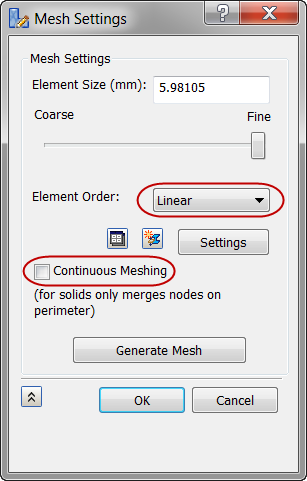
1. Click Mesh Settings from the Mesh panel in the ribbon.
2. Set the Element Order to Linear.
3. Uncheck Continuous Meshing.
4. Click OK to close the dialog and generate the mesh.
5. 
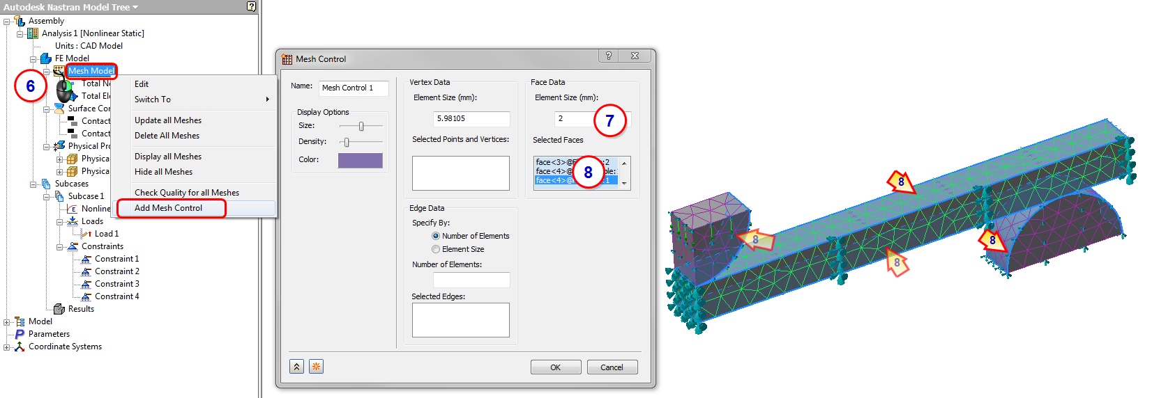
6. From the Analysis tree, right-click Mesh Model > Add Mesh Control.
7. Enter 2 for the Face Data Element Size.
8. Click in the Selected Faces box, and select the four contact surfaces.
9. Click OK.
10. In the Analysis tree, right-click Mesh Model > Generate Mesh.

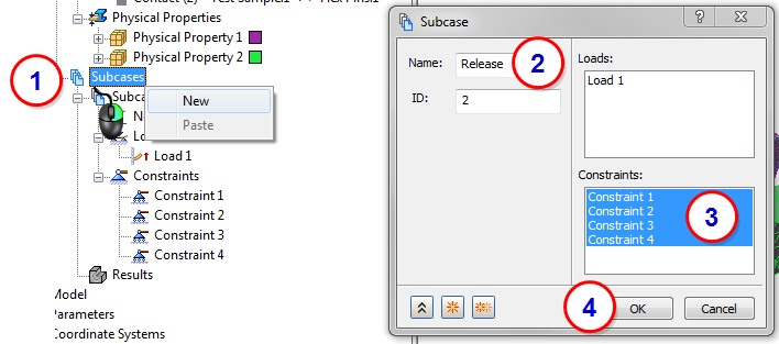
12. Add a "Release" Subcase

1. Right-click Subcases > New.
2. Name the subcase Release.
3. Select the four existing constraints.
4. Click OK.

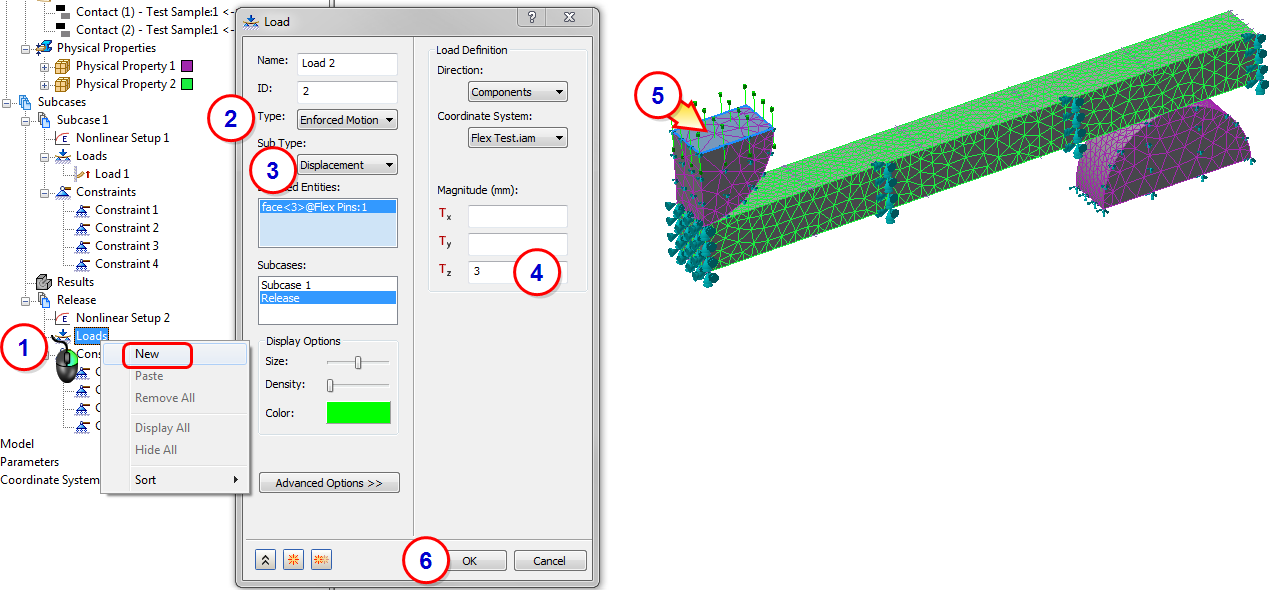
13. Add a Release Load to the Release Subcase

1. In the Release subcase, right-click Loads > New.
2. Set the Type to Enforced Motion.
3. Set the Sub Type to Displacement.
4. Set the Tz value to 3.
5. Select the face shown.
6. Click OK.

14. Define the Nonlinear Setup

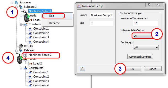
In this step we will enable intermediate output. This provides output data for each load increment.

1. In Subcase 1, right-click Nonlinear Setup 1 > Edit.
2. Set Intermediate Output to On.
3. Click OK.
4. Repeat for the Nonlinear Setup 2 subcase.

15. Run the Model

1. Click Run from the ribbon.

Subcase 1 will solve for 10 load steps.

Subcase 2 will use the results from Subcase 1 as its initial conditions.

16. View the Nonlinear Displacement Results

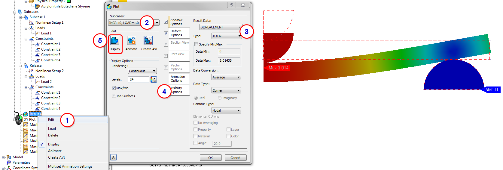
1. From the Analysis tree, right-click Results > Edit.
2. Select INCR 10, LOAD = 1.0 from the Subcases menu.
3. Select Displacement from the Result Data list, and set the Type to Total.
4. Click the Visibility Options tab, and click Hide All.
5. Click Display.

17. View the Nonlinear Strain and Plastic Strain Results

1. Click the Contour Options tab, then select Strain from the Result Data menu, and set Type to SOLID VON MISES STRAIN. Click Display if the results are not showing.



2. Change Type to SOLID EFFECTIVE STRAIN-PLASTIC/NONLINEAR ELASTIC.

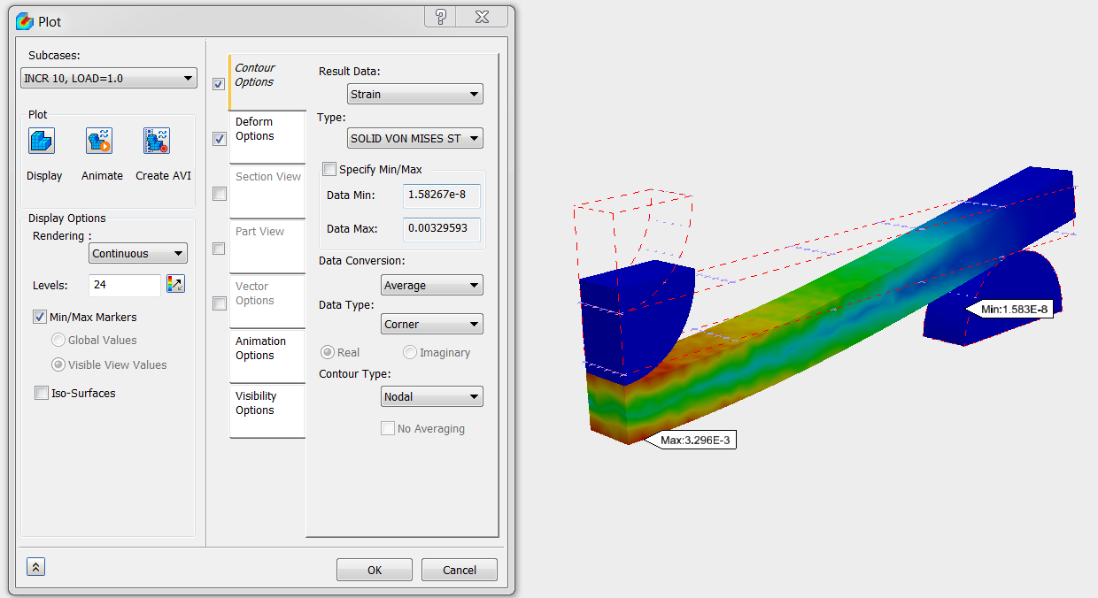
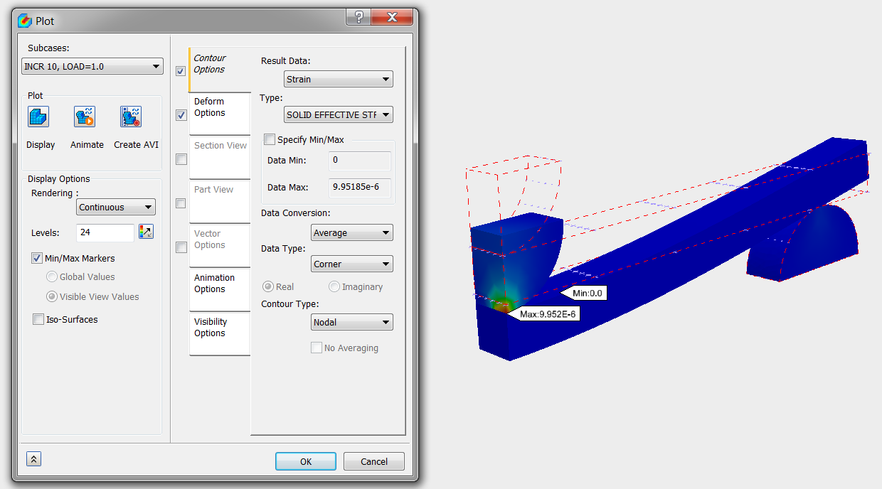
Plastic strain is the strain accumulated beyond the yield strain. Because very little plastic strain is accumulated, permanent deformation to the beam is unlikely.

18. View the Final Deformation

1. Change the Subcase to INCR10, LOAD=2.0
2. Change the Result Data to Displacement.
3. Click Probes from the ribbon, and hover over the end of the beam.
4. Click OK.



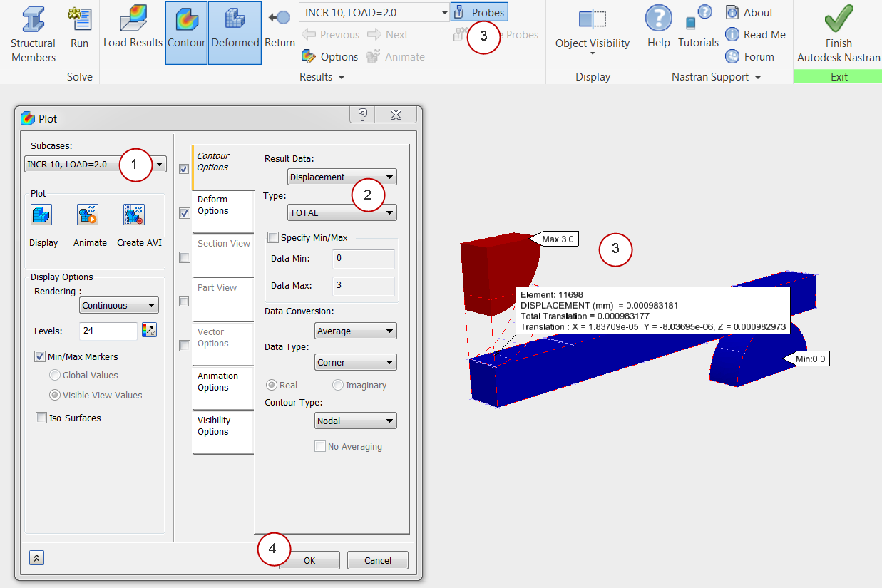
We can see that there is very small amount of permanent displacement in the beam.

19. Create a Multi-Set Animation

1. Right-click on Results, and click Multiset Animation Settings.
2. Set Start Set to INCR 1, LOAD = 0.1.
3. Set the End Set to INCR 10, LOAD = 2.0.
4. Click the Deform Options tab. Set the Deformation Scale to Actual, and the Value to 1.0.
5. Click the Visibility Options tab, and click Hide All.
6. Click Animate.

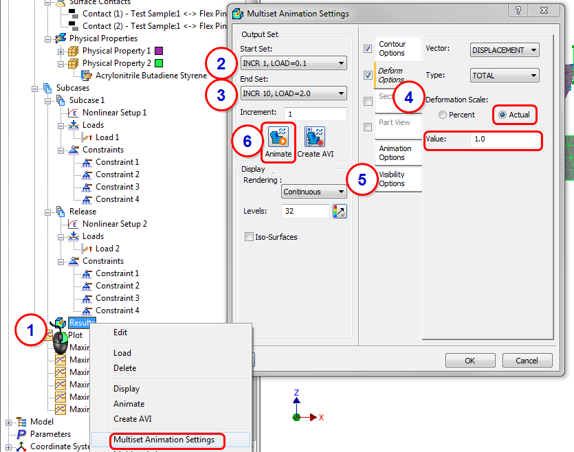
To stop the animation, right-click Results and uncheck Multiset Animate.

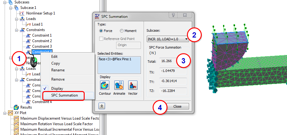
20. Determine the Force Required to Bend the Beam

1. Right-click on the push constraint from Subcase 1, and select SPC Summation. (If you did not name your constraints, click on each until you identify the one assigned to the top of the pin.)
2. Select INCR 10, LOAD = 1.0 as the Subcase.
3. Note the Total Force reported.
4. Click Close.

Summary

In this exercise, we defined a nonlinear material. If we had run this analysis as linear, we would have seen severe nonlinearities that don't appear as severe with the full nonlinear analysis. It is important to understand that even though nonlinear analyses can take longer to solve, running nonlinear is often more physically realistic than running the analysis as linear.

Previous Topic: Nonlinear Materials

Next Topic: Dynamic Analysis