Solution Method
Each of the above governing pdes are discretized using the finite element method described previously. The resulting set of algebraic equations must be solved to determine the values of the dependent variables at the nodes on the finite elements. The algorithm used by Autodesk® CFD to solve these equations is described in this section.
Segregated Solver
The first issue to resolve in solving the discretized equations is that of the missing pressure. If the momentum equations are used to calculate the velocity components, then the continuity equation must be used to determine the pressure. However, pressure never appears explicitly in the continuity equation. There are a plethora of avenues available to circumvent the numerical difficulties with the implicit pressure coupling. Many of these solution methods require that the continuity and momentum equation be solved simultaneously on every node in the finite element mesh. For small problems, this solution is quite adequate. However, for most real-life problems, this solution places a severe penalty on computer resources and in fact may prevent a solution to a problem. To ease this restriction, an equation explicit in pressure must be found.
The pressure equation solved by Autodesk® CFD is derived from the continuity equation. The weighted integral of the continuity equation is taken where integration by parts is used to reduce the order of integration:
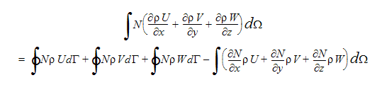
The first three integrals on the right-hand-side (RHS) of this equation represent the mass flux across element boundaries. These integrals will cancel at the interior element faces and will be zero for all boundaries across which no mass flows (symmetry, walls). So these terms represent the natural boundary condition for the pressure equation.
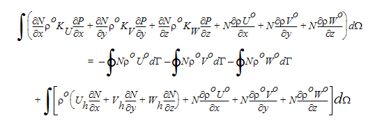
To force the appearance of pressure in this equation, a relationship between velocity and pressure must be derived. This relationship can be deduced from the momentum equations. Using a semi-discretized form of the momentum equations, the velocity-pressure relationship can be written as:
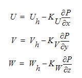
In these equations, the Uh, Vh, Wh terms contain all of the off-diagonal terms in the momentum equations. If these three equations are now substituted into the previous continuity equation, the following pressure equation results:
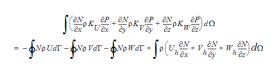
Note that this equation is in the discretized form of the Poisson equation and will therefore produce a symmetric coefficient matrix.
For compressible flow, the density-pressure coupling must also be considered. This coupling is accounted for by using the following expression:
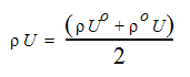
where the o refers to old values. This expression is used when the continuity equation is integrated by parts. Then, substituting for velocity yields:
The extra advection-like terms on the left-hand side of this equation are re-written in terms of pressure using the Ideal Gas Law. With these extra advection terms, the compressible pressure equation will produce a non-symmetric coefficient matrix, much like the other transport equations.
With an explicit pressure equation, each of the governing equations can be solved separately. That is, the x-momentum equation can be solved for U at all of the nodes, the y- momentum equation can be solved for V at all of the nodes, the z-momentum equation can be solved for W at all of the nodes, the pressure equation can be solved for P at all of the nodes, etc. This allows for a much smaller memory requirement since only a single degree of freedom is solved at a time. This approach is called a Segregated Solver because each of the dependent variables are solved separately. In addition, since each of these equations can be solved using iterative matrix techniques, only the non-zero terms in the coefficient matrix need to be stored.