各種變化曲線係用於土木工程,以在切線和圓形曲線之間,以及在兩條具有不同曲率的圓形曲線之間,逐漸引入曲率和超高。
在螺旋線與其他切線和曲線的關係中,每條螺旋線可為內曲或外曲。
工程師在設計和規劃螺旋線時最常用的兩個參數為 L (螺旋線長度) 和 R。R 參數是指螺旋線一端的曲率半徑。R1 和 R2 可用於區分螺旋線起點和終點的半徑。
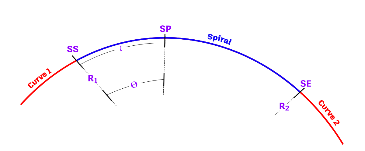
下圖顯示了螺旋線的各種參數:
| 螺旋線參數 | 描述 |
| R1 | 曲線 1 的半徑。 |
| R2 | 曲線 2 的半徑。 |
| SS | 螺旋線起始位置。 |
| SE | 螺旋線結束位置。 |
| SP | 弧長 l 處的螺旋線點。 |
| Θ | 弧長 l 處螺旋線點的中心角度。 |
| l | 從螺旋線起始位置沿螺旋線的弧長。 |
| L | 螺旋線起點和終點位置之間的螺旋線總弧長。 |
複合螺旋線
複合螺旋線提供兩條具有不同半徑的圓形曲線之間的變化。有兩種複合螺旋線:簡單螺旋線和複合螺旋線。複合螺旋線包含由兩條簡單螺旋線組成的曲線。該曲線包含兩個跨距,每個跨距都是一條簡單螺旋線,與其相鄰螺旋線連續相切接合。複合螺旋線允許曲率函數的連續性,並提供在超高中引入平滑變化的方法。
克羅梭螺旋線
雖然 Autodesk Civil 3D 支援數種螺旋線類型,但是克羅梭螺旋線是最常用的螺旋線類型。克羅梭螺旋線在世界範圍內廣泛用於公路和鐵路鐵軌設計。
由瑞士數學家 Leonard Euler 最先研究,克羅梭的曲率函數是線性函數,其將螺旋線與切線相交處的長度函數曲率選擇為零 (0)。然後,曲率將線性增加直到其等於螺旋線和曲線交點處相鄰曲線的曲率。
與簡單曲線不同,它還保持區域曲率的連續性,這在速度較高時會變得更加重要。
公式
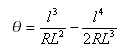
克羅梭螺旋線可以用以下公式表示:![]()
- Θ = 弧長 l 處螺旋線點的中心角度。
- l = 沿曲線的弧長。
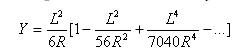
螺旋線的真平度:![]()
螺旋線所對的總角度:![]()
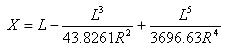
從切線 - 螺旋線點到螺旋線 - 曲線點的切線距離為:
從切線 - 螺旋線點到螺旋線 - 曲線點的切線偏移距離為:
Bloss 螺旋線
可以將 Bloss 螺旋線用作變化,而不使用克羅梭螺旋線。此螺旋線優於克羅梭螺旋線,因為轉換 P 較小,從而會有較長的變化並伴有較大的螺旋線延伸 (K)。此係數在軌道設計中非常重要。
公式
其他關鍵表示式:
從切線 - 螺旋線點到螺旋線 - 曲線點的切線距離為:
從切線 - 螺旋線點到螺旋線 - 曲線點的切線偏移距離為:
正弦曲線
正弦曲線表示連續的曲率路線,適用於切線偏折從 0 度到 90 度的變化。但是,由於正弦曲線比真實的螺旋線更陡,因而很難將其用表格表示並進行監視,所以並未得到廣泛使用。
公式
- Θ = 弧長 i 處螺旋線點的中心角度。
- l = 沿曲線的弧長。
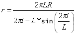
其中 r 為任何給定點處的曲率半徑。
正弦半波長遞減正切曲線
此形式的方程式通常用於日本的鐵路設計。此曲線在變更低偏折角度 (關於車輛動力學方面) 的曲率時需要有效變化的情況下非常有用。
公式
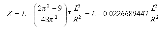
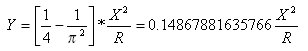
正弦半波長遞減正切曲線可以表示為:
其中,![]() 和 x 是從起點到曲線上任意一點的距離,並沿 (延伸的) 初始切線測量;X 是變化曲線終點處的 X 總數。
和 x 是從起點到曲線上任意一點的距離,並沿 (延伸的) 初始切線測量;X 是變化曲線終點處的 X 總數。
其他關鍵表示式:
從切線 - 螺旋線點到螺旋線 - 曲線點的切線距離為:
從切線 - 螺旋線點到螺旋線 - 曲線點的切線偏移距離為:
三次拋物線
三次拋物線的收斂速度比三次螺旋線稍慢,因而在鐵路和公路設計領域中廣泛使用。
公式
三次拋物線的最小半徑
其中:Θ = 弧長  處螺旋線點的中心角度。
如需參考,請參閱上圖。
三次拋物線根據以下方程式取得最小 r:
所以 ![]()
三次拋物線半徑從無窮大減少到 24 度 5 分 41 秒時的 ![]() ,然後再開始向前增加。這使得三次拋物線無法用於大於 24 度的偏折。
,然後再開始向前增加。這使得三次拋物線無法用於大於 24 度的偏折。
三次 (JP)
此種變化是為滿足日本的要求而開發的。已開發出一些與克羅梭螺旋線近似的螺旋線,以用在偏折角度較小或半徑較大的情況下。這些近似的螺旋線其中之一 (用於日本的設計) 便是三次 (JP)。
公式
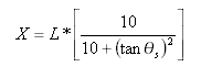
三次 (JP) 可以表示為:
其中 X = 螺旋線 - 曲線點處自切線 - 螺旋線點的切線距離
此公式也可以表示為:

其中 ![]() 為螺旋線處的中心角度 (如插圖 i1 和 i2 中所述)
為螺旋線處的中心角度 (如插圖 i1 和 i2 中所述)
其他關鍵表示式:
從切線 - 螺旋線點到螺旋線 - 曲線點的切線距離為:
從切線 - 螺旋線點到螺旋線 - 曲線點的切線偏移距離為:
NSW 三次拋物線
這是一種滿足新南威爾斯 (澳大利亞) 標準要求的修正的三次拋物線。
公式
NSW 三次拋物線可以表示為:
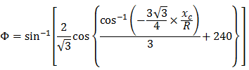


- Φ = R 處最終徑向線與初始切線互垂線之間的角度
- R = 曲線半徑
- Xc = 給定螺旋線的總 X 值
- Yc = 給定螺旋線的總 Y 值
雙二次 (Schramm) 螺旋線
雙二次 (Schramm) 螺旋線垂直加速度的值較小。它們包含兩條二次拋物線,這兩條二次拋物線半徑作為曲線長度 (l) 的函數而變化。
簡單曲線公式
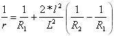
第一條拋物線的曲率:
![]() 其中
其中 ![]()
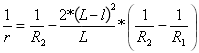
第二條拋物線的曲率:
![]() 其中
其中 ![]()
根據使用者定義的變化曲線的長度 (L) 指定該曲線。
複合曲線公式
第一條拋物線的曲率:
 其中
其中 ![]()
第二條拋物線的曲率:
 其中
其中 ![]()