Thermal problem description
Demonstrate the thermal features within Helius PFA by evaluating a compression loaded plate at elevated temperature.
Four approaches to modeling the material response are used and are designed to highlight important factors that should be considered when including temperature effects in a simulation:
- A temperature dependent material including constituent level thermal residual stresses calculated using material properties at the current temperature environment (EP2_TD_ON_CURRENT_ENV.ans).
- Uses the material created in the previous section.
- A temperature dependent material including constituent level thermal residual stresses calculated using material properties at a specified temperature environment (EP2_TD_ON_SPECIFY_ENV.ans).
- Uses the material created in the previous section.
- A non-temperature dependent material including constituent level thermal residual stresses calculated using material properties at the current temperature environment (EP2_non_TD_ON_CURRENT_ENV.ans).
- Uses a material characterized using the properties at 72°F in the table in the previous section.
- A non-temperature dependent material excluding constituent level thermal residual stresses (EP2_non_TD_OFF.ans).
- Uses a material characterized using the properties at 72°F in the table in the previous section.
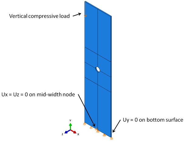
The model consists of a 6 x 1.5 in. plate with a 0.125 in. radius hole located in the center of the plate and uses fully-integrated SOLID185 elements. The layup is [45/-45/0/902]S and the ply thickness is 0.005 in. which results in a plate thickness of 0.05 in. The initial temperature of the plate is modeled at 72 °F and the test temperature of the plate is 140 °F. In the first analysis step, the temperature of the plate is increased to 140 °F. In the second step, a displacement controlled compressive load is applied to the plate until ultimate failure. It is strongly recommended that thermal loads be applied in a step prior to mechanical loading as the thermally induced displacements can cause a large shift in the load-displacement curve, which can make interpretation of the load-displacement curve cumbersome. The loading and boundary conditions are shown in the picture below. In the picture, the 0° ply orientation is aligned with the global y-axis.
The specific initial and final model temperature values are dependent on whether thermal residual stresses are included. If they are included, the initial temperature value must be the actual initial temperature and the final temperature must be the actual final value. This is due to how Helius PFA calculates the ΔT from the stress-free temperature to the temperature of the model. If the residual thermal stresses are not included, the initial temperature of the model should be 0 R and the final temperature should be the ΔT between the temperature the material was characterized at and the final temperature. As an example, the table below lists the initial and final model temperatures for the four models used in the current problem. For further information on the calculation of ΔT, refer to the Thermal Residual Stresses section of the Theory Manual.
| Material | Thermal Residual Stress | Initial Model Temperature | Final Model Temperature | |
|---|---|---|---|---|
| Temperature Dependent | Included (Current Env) | 532 R (72 °F) | 600 R (140 °F) | |
| Temperature Dependent | Included (Specify Env) | 532 R (72 °F) | 600 R (140 °F) | |
| Characterized at 72 °F | Included | 532 R (72 °F) | 600 R (140 °F) | |
| Characterized at 72 °F | Excluded | 0 R | 68 R (=140 °F - 72 °F) |
Input files for each model used in this example problem are available here. If you run any of these files, ensure that the matID in the input file corresponds to the madID for the material(s) that was created here.
Remember, to activate the thermal residual stress feature in Helius PFA, add the *CURE STRESS keyword to the HIN file. To activate temperature dependence, set the 9th HELIUS command argument to a value of -1.0.