DemandWatch Properties dialog

The Properties dialog allows the user to view / edit individual feeds and model parameters for individual feeds. It is also possible from this dialog to test the forecast over a user-defined period and to graphically view results and export them to CSV.

Properties dialog Tabs

The Properties dialog displays the following tabs or pages:

Model Properties - used to view and edit feed properties.
Model Parameters - used to view and edit model parameters.
Forecast Run - used to quickly test the forecast for a time other than the training period to see how the model performs.
Leakage Detection Properties - used to view and edit the properties for detecting probable leaks and possible efficiency improvements.

Model Properties Page

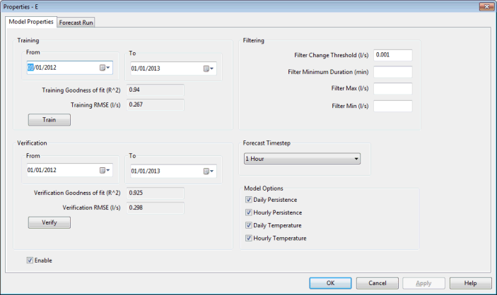
The Model Properties page displays the same information as the corresponding row in the Feeds tab of the DemandWatch Configuration property sheet (values can be edited in the feed Properties dialog or in the Feeds tab of the DemandWatch Configuration object).

In this tab, users can:

Modify training and verification dates
Train and verify feeds
Change filter parameters
Enable / disable feeds on the IWLive Pro server.

Note:

Options available on this dialog are not editable when the related DemandWatch Configuration object is checked-in.

Model Properties tab

The following table lists the options available on this tab:

Training	Training From and Training To define the training period. This period should be at least 12 months span. Training Goodness of fit (R²)- Read only (calculated) field. Variance explained by the training (max is 1). Training RMSE - Read only (calculated) field. Training Root Mean Square Error or accuracy. This parameter measures the difference between training values predicted by the model and the raw values actually measured. The smaller this value the more accurate the training. Train - Click this button to train the feed.
Verification	Verify From and Verify To define the verification period. This period should be at least of 1 month. Verification Goodness of fit (R²) - Read only (calculated) field. Variance explained by the verification (max is 1). Verification RMSE - Read only (calculated) field. Verification Root Mean Square Error or accuracy. This parameter measures the difference between values predicted by the model and the raw values actually measured. The smaller this value the more accurate the verification. Verify - Click this button to verify the feed.
Filtering	Filter Change Threshold - Threshold defining a change in flow values. If the change in the incoming data during the Filter Minimum Duration is less than the threshold, the incoming data is discarded (value difference is considered to be negligible). In other words, if the data flat-lines the incoming data is discarded as long as the change in the data during the flat-lining is less than the filter change threshold. Filter Minimum Duration - Minimum duration after which a data feed value that is not considered to have changed compared to the initial value (see Filter Change Threshold above) will be discarded. Filter Max - Maximum flow value allowed. Data values equal to or larger than the filter max will be discarded. Filter Min - Minimum flow value allowed. Data values equal to or less than the filter min will be discarded.
Forecast Timestep	Demand forecast timestep. Available values are 5 mins, 10 mins, 15 mins, 20 mins, 30 mins, 1 hour and 2 hours. Note: If the demand forecast timestep is modified for an existing model, it is necessary to re-train that model.
Model Options	Model options section allowing users to fine tune their model. In here can be set the short term memory components to be used. In the case of temperature data being included in the regression, it is also possible to set whether the temperature feed specified in the Feeds page of the DemandWatch Configuration object for this individual feed is to adjust the demand forecast daily or hourly. Daily Persistence - Use the 24 hour short term memory component (PSI24). Hourly Persistence - Use the 1 hour short term memory component (PSI1). Daily Temperature - Use the specified temperature feed to adjust the daily demand forecast values. Hourly Temperature - Use the specified temperature feed to adjust the hourly demand forecast values. Enable options as appropriate, to use them during training and forecast.
Enable	Check this option to enable the feed so it is used in forecast runs by the IWLive Pro server.

Model Parameters Page

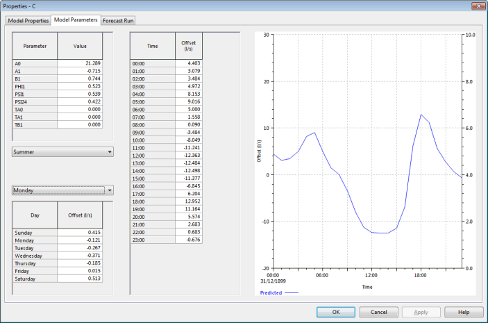
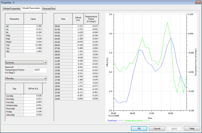
The Model Parameters page allows users to adjust model values (offsets, parameters, season and weekdays) and to view them graphically.

Tip:

This page is hidden by default and can be shown by enabling the Show Details Model Parameters Page option of the Options dialog.

InfoWorks WS Pro is based on the short-term, pattern-based model for water-demand forecasting developed by Alvisi, Franchini and Marinelli (2007)¹. Please refer to this article for more information on the model and its components.

Note:

Options available on this dialog (with the exception of season and weekday selection) are not editable when the related DemandWatch Configuration object is checked-in. It is not recommended that users edit model parameters.

Model Parameters tab

Example of Model Parameters page for a telemetry feed

Model Parameters tab

Example of Model Parameters page for a temperature feed

The following table contains the model parameters present on this tab:

Option	Description
Model short-time components	AO, A1 and B1 are Fourier series components. See equation (2) of Alvisi, Franchini and Marinelli (2007)¹. PHI1 - 24-hour short term memory for the daily component. See equation (6) of Alvisi, Franchini and Marinelli (2007)¹. PSI1 - short term memory for one hour for the hourly component. See equation (10) of Alvisi, Franchini and Marinelli (2007)¹. PSI24 - short term memory for 24 hours for the hourly component. See equation (10) of Alvisi, Franchini and Marinelli (2007)¹. TA0, TA1 and TB1 are Fourier series coefficients for the temperature feed that are used to calculate the expected daily temperature for a particular day. Note: TA0, TA1 and TB1 only apply to temperature feeds and will be equal to zero for telemetry feeds.
Season	Season drop-down list. Select a season.
Seasonal Temperature Factor	Available for temperature feeds only. This parameter indicates the increase in average daily demand per increase in temperature for each season. For example, if the seasonal temperature factor is 1.0 l/s/^oC, for every degree temperature increase, the average daily demand will increase by 1.0 l/s.
Weekday	Day drop-down list. Select a day.
Daily offsets	Displays the day offsets for the selected season in a tabular form.
Hourly offsets	Displays the hourly offsets for the selected season and day of the week in a tabular form.
Temperature Factor	Available for temperature feeds only. Displays the hourly temperature factor for the selected season and day of the week in a tabular form.
Graph	Graphical representation of the hourly offset data for the selected season and day.

Forecast Run Page

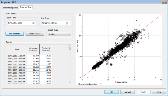
The Forecast Run page allows users to run forecasts between given dates. Results are subsequently displayed on the tab in tabular and graphical form.

Forecast Run tab

The table below shows detailed information on the data available in this tab:

Option	Description
Time Range	Enter a Start Time and an End Time for the forecast run.
Run Forecast	Click this button to run the model for the selected time range.
Export to CSV	Click this button to export the results of the test forecast run to a CSV file. This will display a standard Windows File Save dialog.
Graph type	Type of graph to use for the results. Normal (Default) - flow vs date/time. Scatter - scatter graph (predicted vs measured).
Results	Results of the forecast run (measured and predicted values) presented in a grid.
Graph	Graphical representation of the results displayed in the grid. Type depends on the setting of the Graph type field.

Reference:

¹ Alvisi S., Franchini M. and Marinelli A. (2007). A short term pattern-based water demand forecasting model. Journal of Hydroinformatics, 09.(1), pp. 39-50, 2007. IWA Publishing.