Amplitude curves in quasi-static event simulations
In Quasi-static studies, the concept of time is dimensionless. Time is simply a pseudo time that measures the application of the transient loads and prescribed boundary conditions.
If you know the load values, apply transient loads and enable Step Dependent to activate the Magnitude Curve.
If you don't know the loading values but you know the displacement under load, use the prescribed constraint and let the solver figure out the load required to create that displacement, using the steps you specify in the Multiplier Curve.
Duration and amplitude
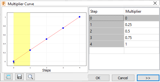
You specify the number of steps for the simulation and provide amplitude curves that describe the transient load (magnitude curve) and prescribed displacement (multiplier curve) boundary conditions over those steps.

Figure 1. Example multiplier curve showing multiple steps.
Analysis time considerations
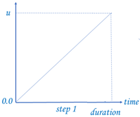
The default number of steps is one, which is appropriate for a loading that is monotonic. In this case, you prescribe the loads and boundary conditions with a linear ramp from zero to one.

Figure 2: Load problem with a linear up ramp.
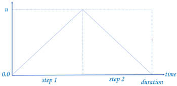
If your loading is not monotonic, specify how many steps the solver should use. For example, you may want to load the model up to some prescribed value and then unload it back to zero. This simulation would use two steps.

Figure 3: Load/unload problem with a linear up/down ramp.