This section presents how a Bifrost Object is populated to express a Bifrost Geometry.

Quick Reference

1. Geometry is defined by [Geo Properties] on a Bifrost Object
2. [Geo Properties] can define components (point_component), data (e.g. point_position or face_offset), or ranges (face_vertex_normal_index).
3. Data geo properties may target components directly or have indirection.
4. Schemas define what geo properties are necessary for an object to be a certain type of geometry (e.g., a mesh).

The quick reference guide shows the names and targets of the geo properties which comprise the structure of the geometry.

Points

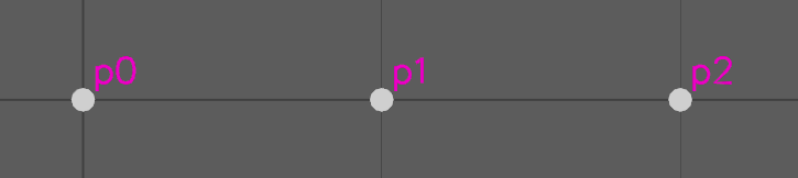
The point indices are shown next to the points.

point_component:  count: 3

point_position:   target: point_component
                  data: [{0,0,0}, {1,0,0}, {2,0,0}] (array<float3)

Points have only one component, point_component.

See sdk/examples/TwistDeformer in your installation for an example of point's manipulation.

Strands

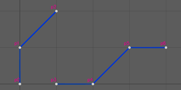
The point indices are shown next to the points.

point_component:  count: 7
strand_component: count: 2
strand_offset:    target: strand_component
                  data: [0, 3, 7] (array<uint>)

point_position:   target: point_component
                  data: [{0,0,0}, {0,1,0}, {1,2,0}, {1,0,0}, {2,0,0}, {3,1,0}, {4,1,0}] (array<float3>)

Strands are points, with an offset array to define strands.

strand_offset is an array over the strands* which specifies at which point each strand starts and ends.

Mesh

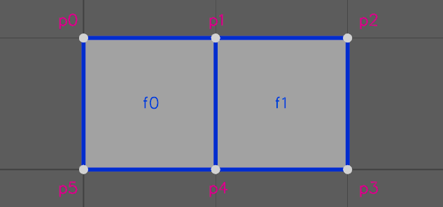
The point indices are shown in the white circles. The face indices are show in the center of each face. The face vertex indices are shown at the corners of each face.

point_component:        count: 6
face_component:         count: 2
face_vertex_component:  count: 8
face_offset:            target: face_component
                        data: [0, 4, 8] (array<uint>)
face_vertex:            target: face_vertex_component
                        data: [0, 5, 4, 1, 1, 4, 3, 2] (array<uint>)

point_position:         target: point_component
                        data: [{0,1,0}, {1,1,0}, {2,1,0}, {2,0,0}, {1,0,0}, {0,0,0}, ]

Meshes are points, with face and face_vertex data to create faces.

face_offset is an array over the faces* which specifies at which face_vertex each face starts and ends. face_vertex is an array over the face vertices which specifies which point is at each face_vertex.

See sdk/examples/MeshArea and sdk/examples/ObjWriter in your installation for some examples of mesh manipulation.

Geometry Data Structure

Geo Properties

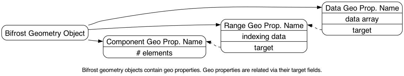
Geo Properties define geometric features. There are three types of geo properties:

• Component Geo Properties: These describe the topological features of a geometry. For example the points on a particle system or faces on a mesh.
• Data Geo Properties: These describe data which is attached to the components of the geometry (i.e. point positions, normals, weights, velocities, etc.).
• Range Geo Properties: These describe mappings from one range of values to another. For mesh data specifically, they store indices for indexed data like UVs, i.e. they map a range of component values (0 to the # of face vertices) to a range of UV values (0 to the number of elements in the UV array).

For example, Points contain at least two geo properties. One point_component component geo property to declare a points topological feature, and a point_position data geo property to define the actual local-space positions of the points.

A geometry object is one that contains one or more geo properties, as shown below:

Geo Property Targets

Data and Range geo properties contain a target property that define a relationship between the geo property and the topological components. Most data geo properties target components directly. The data geo property is trivially mapped onto the topological component its targeting with a 1:1 mapping.

For example, a points geometry will have a point_position data geo property that targets the point_component. For each point i, the associated point_position is found in the point_position's data array at index i. The point_position array must contain at least as many elements as specified in the point_component's count field.

In the graph, the get_geo_property and set_geo_property nodes are used to get and set the data arrays of geo properties. With the C++ API, equivalent functions are available to set and set the data arrays of geo properties, for example Bifrost::Geometry::getDataGeoPropValues, Bifrost::Geometry::setDataGeoPropValues and several other functions can be found in the API reference section.

A points geometry with five points, with positions starting at (0,0,0) and ascending to (0,4,0) would look like this:

point index:         0        1        2        3        4
point_position: [ (0,0,0), (0,1,0), (0,2,0), (0,3,0), (0,4,0) ]

Indexed Geo Properties

Range geo properties represent index arrays that provide an additional level of indirection between the topological components of the geometry and a corresponding data geo property data array. They are useful in two cases, when there are shared data elements, or the identity of the data elements is important and not just the value.

In practice, mesh normals and UV coordinates typically use indexed geo properties.

In the case of mesh normals, it is very commonly the case that most normals are smooth. For example, on a cylinder, only the border between the caps and the sides unsmooth normals. Each point on the sides (aside from the edge of the caps) of the cylinder connects to four face vertices but they all have the same normal. This data can be shared to save memory. This is expressed in the same way, where face_vertex_normal data geo property targets the range geo property face_vertex_normal_index, which in turn targets face_vertex_component.

For UV coordinates a float2 array of coordinates is stored in a data geo property named face_vertex_uv, which targets a range geo property named face_vertex_uv_index. face_vertex_uv_index is the range geo property which contains the index array. The range geo property then targets the face_vertex_component. For UV coordinates in particular the identity of the referenced UV coordinates is important. Face vertices that reference the same vertex but different UV coordinates represent UV seams (also called UV borders) within a mesh.

face_vertex_uv      -> face_vertex_uv_index       -> face_vertex_component
face_vertex_normal  -> face_vertex_normal_index   -> face_vertex_component

As a simple example, adding an indexed point_weight property to our previous example might look like this:

point index:             0        1        2        3        4
point_position:     [ (0,0,0), (0,1,0), (0,2,0), (0,3,0), (0,4,0) ]
point_weight_index: [    0   ,    0   ,    1   ,    1   ,    2    ]
point_weight:       [ 10, 20, 30 ]

point_weight_index contains an index array, and point_weight contains the actual weight values of the points. Note that the point_weight_index array has five elements, matching the number of points. Also, note that each element contains a value between 0 and 2. These values are the indices into the point_weight array. In our example there are only three point weight values so the point_weight array contains only three elements. Note that this is less than than the number of points. Data arrays of indexed geo properties will typically be smaller than the component they target. To find the point_weight for a given point i, find the value of point_weight_index[i] and use it to look up a value in the point_weight array. For example, the point_weight for point 4 would be the point_weight element at point_weight_index[4] which is 2. Thus the point_weight for point 4 is point_weight[2] which is 30.

See sdk/examples/MeshWeldUV in your installation for an example of Indexed Geo Properties manipulation.

Indexed Properties in the Graph

get_indexed_geo_property and set_indexed_geo_property are provided to get and set both the data and index arrays for a geo property at once.

Indexed Property Targets

Note that component geo properties do not have a target property, and data geo properties may not be targeted by any other geo properties. Therefore the data and component geo properties always form the beginning and end, respectively, of a target chain. Finally, targets resulting in a circular dependency are not allowed, nor can geo properties target themselves.

Offset Arrays

An offset array is a memory-efficient method to pack 2d data into a 1d array. In Bifrost offset arrays are used to define which points belong to individual strands within a strands geometry or individual faces in a mesh geometry. Instead of a separate array for each strand or face the point data is packed into a single 1d array and the offset array stores a series of offsets into this data array. There is one offset for each individual strand or face, plus one additional element at the end. The value of this extra element is the size of the data array. Its usage is described in more detail below.

Recall from the quick reference this strands geometry that contains 7 points, and 2 individual strands lying on the xy-plane.

point_component:  count: 7
strand_component: count: 2
strand_offset:    target: strand_component
                  data: [0, 3, 7] (array<uint>)

point_position:   target: point_component
                  data: [{0,0,0}, {0,1,0}, {1,2,0}, {1,0,0}, {2,0,0}, {3,1,0}, {4,1,0}] (array<float3>)

The point_position array contains 7 values. They correspond to the corners and end points of the strands. There are 2 strands, therefore the strand_offset array would contain 2 + 1 = 3 elements. One element for each strand, plus one extra element pointing to one past the last point:

point index:          0,       1,       2,       3,       4,       5,       6
point_position:   [{0,0,0}, {0,1,0}, {1,2,0}, {1,0,0}, {2,0,0}, {3,1,0}, {4,1,0}]
                   |                         |                                  |
                   |<------- strand[0] ----->|<----------- strand[1] ---------->|

In this case strand 0's offset is strand_offset[0], which is 0. Thus the range of points it references starts at point 0. Strand 1's offset is strand_offset[1] which is 3. Thus the range of points it reference starts at point 3. To determine the number of points each strand uses, subtract the next strand's offset from the current strands offset.

For example to determine how many points strand 0 references:

point_count = strand_offset[1] - strand_offset[0] = 3 - 0 = 3

And for strand 1:

point_count = strand_offset[2] - strand_offset[1] = 7 - 3 = 4

In general for a single strand s, the number of points it references is given by:

point_count = strand_offset[s+1] - strand_offset[s];

Recall that the offset array contains one extra element at the end. The extra element allows this formula to work correctly even when s is the last strand.

The range of points that each strand references is given by:

point_start_index = strand_offset[s]
point_end_index = strand_offset[s+1]

Note that point_end_index is one past the last point index referenced by s.

Schemas

Schemas are how geometry types in Bifrost are defined, in terms of what geo properties are required for a Bifrost object to qualify as, for example, a mesh. Note that both also satisfy the points schema, though the inverse is not true.

Points Schema

Points, or point clouds, are defined by the points.json schema file. They are the simplest type of geometry. They consist solely of points, and their positions in space. They are composed of two geo properties:

• point_component: Component geo property that represents the point topological component.
• point_position: Data geo property that stores the array of 3D point positions. There is one element in this array for each point component.

Points can be used to represent point clouds, particle systems, and other simple data structures. However, they are also the basis for more complex geometry types. Strands, Meshes, Instances can all be considered Points objects with additional data.

Strands Schema

Strands are defined by the strands.json schema file. A single strand represents a collection of connected points. A strands geometry object is a collection of individual strands. They are composed of four geo properties:

• point_component: Component geo property that represents the point topological component.
• strand_component: Component geo property that represents the strand topological component.
• point_position: Data geo property that stores the array of 3D point positions. There is one element in this array for each point component.
• strand_offset: Data geo property that stores the array of offsets into the point_position array for each strand. This data array size is equal to the number of strand_components plus one. The last element contains an index to one past the last element in the point_position array. See below for an example.

Meshes Schema

Meshes are defined by the mesh.json schema file. They are composed of six geo properties:

• point_component: Component geo property that represents the point topological component.
• face_component: Component geo property that represents the face topological component.
• face_vertex_component: Component geo property that represents the face vertex topological component.
• point_position: Data geo property that stores the array of local space positions of the points. This data array size is equal to the number of point_components.
• face_vertex: Data geo property that stores the array of point indices for each corner of each face. This data array size is equal to the number of face_vertex_components.
• face_offset: Data geo property that stores the array of offsets into the face_vertex array for each face. This data array size is equal to the number of face_components plus one. The last element contains an index to one past the last element in the face_vertex array. See below for an example. Note that the mesh format uses a counter-clockwise face-winding order.

Mesh Example

This example defines two triangles lying on the xz-plane. The two triangles share an edge. In the diagram below, the points are labeled 0-3, and the faces are labeled 0-1.

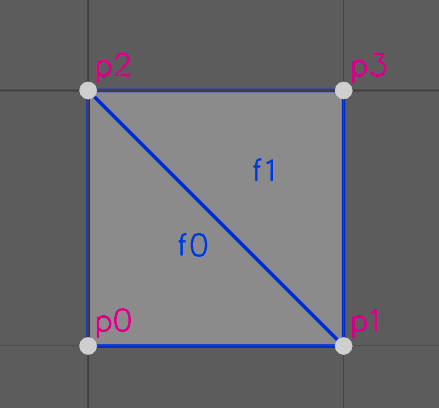
point_component:        count: 4
face_component:         count: 2
face_vertex_component:  count: 6
face_offset:            target: face_component
                        data: [0, 3, 6] (array<uint>)
face_vertex:            target: face_vertex_component
                        data: [0, 1, 2, 1, 3, 2] (array<uint>)

point_position:         target: point_component
                        data: [{0,0,1}, {1,0,1}, {0,0,0}, {1,0,0}]

The point_position array contains 4 values. They correspond to the white dots in the diagram.

There are 2 faces, and each face references 3 points, therefore the face_vertex array would contain 3 + 3 = 6 elements. 3 elements for the first face, and 3 elements for the second face. The first face, labeled with 0, references points 0, 1, and 2. And the second face, labeled 1, references points 1, 3, and 2.

The face_offset array contains offsets into the face_vertex array. It specifies the range of elements in the face_vertex array that correspond to each face. In this example the elements in the face_vertex array that correspond to face 0 are the range [0,3). i.e. face_offset[0] and face_offset[1]. For face 1, the corresponding face_vertex elements are in the range face_offset[1] and face_offset[2]. In general, the corresponding face_vertex elements for face n are in the range face_offset[n] and face_offset[n+1].

Note that face_offset array contains one more element than the number of faces. This is to allow the above algorithm to work without modification for the last face. See the Offset Arrays section of this document for more details.

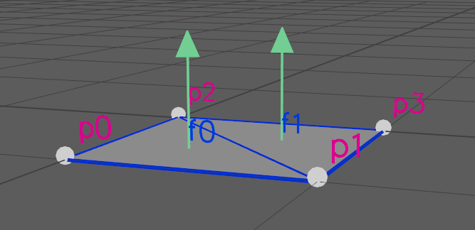
Counter-Clockwise Winding Order

The ordering of values in the face_vertex array is important. The front side of a face is determined by the ordering of its face vertices. This ordering is called the winding order of the face. In the previous example, the first triangle's indices are 0, 1, 2. This ordering lists the face vertices counter-clockwise around the face relative to the viewer. Thus, the front side of the face is pointing towards the viewer. If the ordering of the face vertices is changed to 0, 2, 1, then they would be listed in clockwise ordering relative to the viewer, and the front side of the face would point away from the viewer, into the screen.

The front side of the face is the side that the face's normal will point. Typically each face's winding should be consistent with its neighbors. In the previous example, both triangles have the same counter-clockwise winding so their face normals (shown as green arrows) point in the same direction:

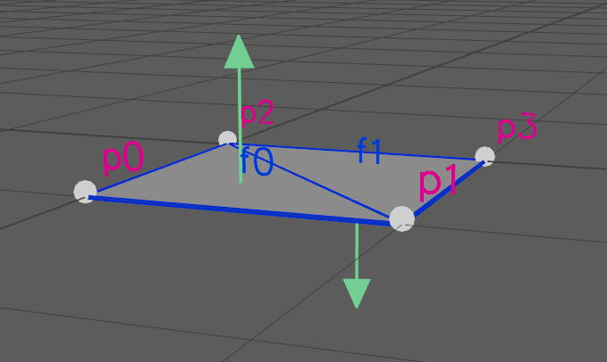
If the second triangle's face vertices are changed to 2,3,1 its face normal would point in the opposite direction as the first triangle. Meshes with inconsistent winding orders should be avoided:

Mesh Adjacency

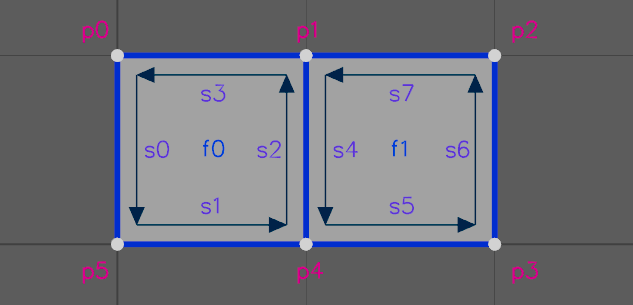
Faces are adjacent to each other if they share a common edge. A point is adjacent to all of the faces that reference that point. The corners of a face are the points referenced by that face, relative to the face. The sides of the face are the called the face edges between successive corners. For example, given the mesh:

    face_offset = [0, 4, 8]
    face_vertex = [0, 5, 4, 1, 1, 4, 3, 2]

f0 references points [p0, p5, p4, p1] and f1 references [p1, p4, p3, p2]. Each face references 4 points. Thus they both have 4 corners and 4 sides. The sides and corners of each face are labelled below:

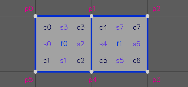
Since f0 references points [p0, p5, p4, p1] corner c0 corresponds to p0, c1 corresponds to p5, etc. Side s0 is the side of the face between corner c0 and c1. Similarly s1 is the side of the face between c1 and c2, etc. Note that the sides are directed. They start from the corner with the lower index to the corner with the higher index. i.e. s[i] is defined as the half-edge from c[i] to c[i+1]. The only exception is the last side, which will go from the last corner to the first corner (i.e c[n-1] to c[0] for a face with n face vertices).

For example, face f0, side s2 is adjacent to face f1, side s0 in the above mesh because both (f0, s2) and (f0, s0) reference the same pair of points: p1 and p4. If a side of a face has no adjacent face, it is considered an open edge.

In Bifrost a face and a side/corner within that face is called a face edge. The FaceEdge data type represents this concept in the graph. It contains two indices. One for the face, and one for the side/corner within that face. Use the update_mesh_adjacency node to compute the adjacency for every face edge within the mesh.

The direction of each face edge in the above example is labelled below:

Note that (f0, s2) runs in the opposite direction of its adjacent face edge, (f1, s1). This is a natural result of the two faces having the same counter-clockwise winding order. If the two faces had different winding orders, then the face edges in each face would run in the same direction. See the section Counter-Clockwise Winding Order in this document for more details.

The update_mesh_adjacency node also computes the adjacency for every point in the mesh. For point p0, the only adjacent face is f0, and the corner within that face that references p0 is c0. For p1, there are two adjacent face/corners, (f0, c3) and (f1, c0). The number of adjacency values for each point depends on how many faces reference that point.