
The explicit dynamics method is ideal for modeling highly nonlinear, large-deformation, contact-dominated problems that involve impact, multi-body contact, and highly nonlinear material behavior.
In general, performing nonlinear explicit simulations is often simpler than performing linear simulations. The user has no "convergence" settings to tweak, as is necessary for linear solvers, and simply launches the simulation without regard for the linearity of the system.
The explicit dynamics procedure is ideally suited for simulating extremely large models regardless of how nonlinear the problem might be. The key enabler is that there is no assembled system of algebraic equations that must be solved for each time step as you find in traditional implicit finite element formulations.
An explicit solver simply forms the dynamic equilibrium equations for the finite element model at each instance in time and uses an explicit integration rule to march forward in time. In a nutshell, not having to solve large systems of algebraic equations means a small memory footprint and each time step is extremely efficient to compute. We will see that the explicit algorithm requires a relatively small time step, so it is extremely important that the cost of each times step is low.
Material deletion
Autodesk Explicit allows you to define material deletion criteria that governs material failure and thus removal from the simulation. This is done by simply defining a maximum value for various strain measures that the material cannot exceed. Once the user-defined criteria is satisfied at a finite location in the model, Autodesk Explicit removes the material at that location and deletes the corresponding element from the mesh. Typical strain measures for deletion include equivalent plastic strain and maximum principal strain.
When material deletion is utilized in a simulation, Autodesk Explicit accounts for the erosion of finite elements by continuously updating the contact surfaces to consider newly exposed regions of the model. Material deletion coupled with contact surface erosion allows you to tear your model apart and blow holes in it.
Rigid bodies
With a single declaration, you can specify that a part of the model is rigid. As a result, Autodesk Explicit will automatically compute the center of mass and all the rigid body properties for the part (e.g. mass moments of inertia and total mass) and compute the response of the part using rigid body dynamics equations. Since the part is rigid, it will not deform locally meaning there will be no stress or strain in the part. Contact conditions will automatically be maintained between parts irrespective of whether or not a part is rigid. Best of all, rigid parts do not participate in the determination of the stable time step.
Contact
Contact modeling is very straightforward within the explicit dynamics technology. You simply define all the parts that make up your assembled model and the application will automatically monitor the collisions between the parts and enforce kinematic compliance. There is no limit on the number of parts that can contact one another and very little effort is required by the user.
At most, the user specifies friction behavior between the different parts (default friction coefficient is zero) or specifies that the contact surfaces are welded together (default behavior is non-welded/separable surface pairs). Autodesk Explicit constantly monitors and tracks the proximity of the various free surfaces of the model though all the large deformations and rotations to enforce the kinematic compliance of the parts when collisions are detected.
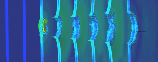
One of the most versatile features of the contact detection algorithm is that it will automatically rebuild the surfaces of the model as material erosion occurs and new surfaces are exposed due to element deletion. Figure 2 demonstrates a simulation of a bird strike on a turbine.
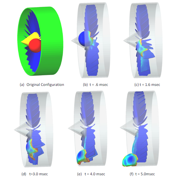
Figure 2: Example of Automatic Contact Tracking
The "bird" is modeled as a sphere comprised of a soft plastic material and it impacts the turbine at 300 mph. The turbine blades are steel and the turbine is spinning at 6000 RPM. The automatic contact monitors collision between the sphere and the blades, and also all of the blades with one another. The sphere and the blades are also monitored for contact with the outer shroud. The spherical bird has material deletion criteria based on plastic strain with a value of 30%. The steel turbine blades have material deletion criteria based on plastic strain of 100%.
As the sphere impacts the blades, the sphere heavily deforms and material erosion occurs. At each time step during the simulation, all of the contact surfaces are rebuilt automatically. Note the leading edge of the blades also experience erosion, so Autodesk Explicit is simultaneously rebuilding two eroding parts that are presently in contact. All of the collision detection and surface rebuilding is automatic and requires no user intervention.
Explicit integration
The key to the versatility of the explicit dynamics procedure is the integration algorithm from which it takes its name. At time t, the finite element solver calculates all the forces on the mesh from both the internal forces (due to the stresses in the elements) and the external forces (due to the applied loads).
Acceleration(t) = [External Forces(t) – Internal Forces(t)]/Nodal MassThe secret ingredient that makes explicit dynamics so efficient is that we use a lumped nodal mass. This means that we can compute all the nodal accelerations without resorting to any kind of linear algebraic solver. Once we know the accelerations at time t, we explicitly integrate forward in time the nodal values of the accelerations to obtain the nodal values of velocities and displacements at time t+Δt:
Velocity(t + Δt) = Velocity(t) + Δt•Acceleration(t)
Displacement(t + Δt) = Displacement(t) + ½Δt•[Velocity(t) + Velocity(t + Δt)]
What could be easier than that? All the real computational effort appears in the step to compute the internal and external nodal forces, which is where all the finite element methodology occurs, but even there we only perform a fraction of the finite element calculations found in a conventional implicit finite element solver. With the explicit approach we only form the right-hand-side of the equations of motion.
With an implicit solver, however, you form the same right-hand-side but you also must assemble the global stiffness matrix and directly solve the system of equations. For nonlinear models, an implicit solver must re-form, re-assemble, and re-factorize the global system matrix at every time step. Here we see very clearly why explicit dynamics solvers are so efficient at nonlinear simulations. Every explicit time step is literally orders of magnitude faster than an implicit time step!
Since every time step in explicit dynamics spends the vast majority of the computational time in the formation of element forces, the actual runtime for your simulations is directly proportional to the number of elements in the model. You would expect then that, if you refine the model by say a factor of 2 in every direction so you have 8 times as many elements, it would take 8 times longer for the solution. However, it would actually take 16 times longer, because the time step size will be half the size of the unrefined model.
Automatic time stepping controlled by stability limits
Of course, if something sounds too good to be true, there is usually something more to the story. In this case, the explicit integration method described above is governed by a stability limit. Simply put, there is a critical time step size that you cannot exceed while performing explicit integrations. This is known as the stability limit and it depends upon your mesh sizing and your material properties.
If you are performing a dynamic simulation using a conventional implicit solver, you typically specify the duration of the response you want to calculate and the number of time steps to use. For example, you might want a simulation duration of one second using 100 time steps, in which case your time step size is .01 seconds and it remains fixed throughout the analysis. But when you run an explicit dynamics simulation all you are allowed to specify is the total time duration. The explicit dynamics solver automatically picks the time step size to remain below the stability limit of the model. You have no control over the number of time steps the explicit solver will take!
So how is the stability limit determined? There is lots of very complicated mathematics that goes into precisely determining the stability limit for your model. The correct technical answer is that it depends upon the highest natural frequency in the model. But we have a simple way to think of this in terms of the size of your elements and the wave speed in your materials. We can compute the critical time step for each element as the time it takes to transmit a wave across the length of the element (i.e. the element length/wave speed). The critical time step for the simulation is simply the smallest value for all the elements of the mesh.
Wave speed is computed by taking the square root of the ratio of the material modulus and the material density. There are several different wave speeds (e.g. longitudinal, shear, dilatational, etc.). For the purposes of illustrating this concept we will use the longitudinal wave speed based upon Young's modulus (the precise mathematical form found in Autodesk Explicit is the dilatational wave speed). For a steel material model with Young's modulus of 200 GPa and density of 7800 N/m3 the wave speed is about 5000 m/sec. A very large number indeed! Every element in the mesh has some characteristic length associated with it. We will not try to be particularly precise here; let's just assume the characteristic element length is the shortest edge on the element. So, if you have elements that are of size 1 mm in your steel part, your time step in the explicit dynamics will be something like 2•10-7 sec.
Yes, the time step is less than a microsecond! This is quite common in explicit dynamics, you are going to take a lot of time steps! But every time step is performed in a very efficient manner, so the total runtime is also efficient.
Figure 3 shows a sketch of a dilatational wave propagating across a non-uniform mesh.
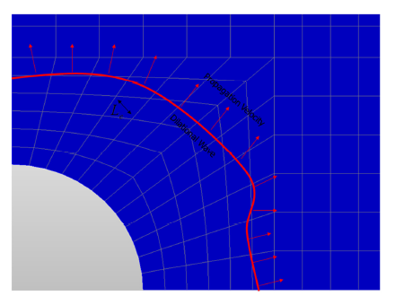
Figure 3: Dilatational wave propagation in a mesh
Every element has some characteristic length that we show generically in the figure as x0007. Every element in the mesh knows its current value for the dilatational wave speed in the material at that point (the material wave speed can actually change in nonlinear material models). It does not matter where the wave is at any particular time. In fact, there are lots of waves running around the mesh! The explicit procedure simply computes the transit time across every element and takes a time step that corresponds to the minimum value over the entire model.
The important thing to keep in mind is that you, the user, don't have to keep track of any of this. Autodesk Explicit is constantly monitoring the stability limits of the model and choosing the time step for you as the simulation progresses.
Key points to remember about the stable time step size are as follows:
- The stable time step is directly proportional to the element sizes. Refining your mesh by a factor of 2 will reduce the time step by a factor of 2.
- The runtime for your model is directly proportional to the number of elements in the model, as well to the number of time steps you will take to integrate the response over the duration. Refining the mesh by a factor of 2 in every direction will increase the number of elements by a factor of 8, but the runtime will take 16 times longer!
- The stable time step is directly proportional to the square root of your material modulus. Very hard materials like steel will have a smaller stable time step than soft materials like rubber.
- The stable time step is inversely proportional to the square root of your material density. Heavier materials have a larger stable time step since it takes more time for a wave to propagate across a material with greater mass.