
Transient Boundary Conditions
Most of the boundary conditions in Autodesk® CFD can be made to vary with time. This is useful for simulating the effects of increasing or decreasing the amount of flow, pressure, or energy is coming into the device.
To make a boundary condition vary with time, begin by opening the Boundary Conditions quick edit dialog. (Click Edit from the Boundary Conditions context panel):
- Change the Time to Transient on the boundary condition dialog.
- Select the Time Curve method and specify the parameters on the pop-out dialog. There are seven methods for varying a load with time.
- Check the variation by clicking the Plot button. This is helpful to ensure that the variation works as intended.
Constant
The Constant variation method keeps the value constant throughout the analysis. This is equivalent to assigning a steady-state boundary condition.
A typical use for Constant would be as a place-holder for a different transient condition later in the analysis. One might initially assign a constant value as a transient condition and later change it to a different variation method.
Ramp Step
The Ramp-Step function combines a linear ramp function with a flat step function:
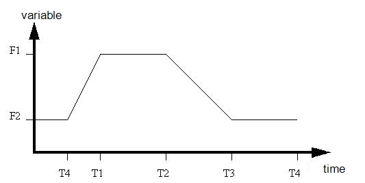
The T values are the times that inflections occur.
The F values are the min and max of the variables.
- Specify the function so that the maximum value (F1) occurs first at time T1.
- At time T2, the value starts to ramp down.
- At time T3, the function hits its minimum value (F2).
- At time T4, the value starts to ramp up.
Periodic
The Periodic type of boundary condition is exponential in time. The functional form is:
F(t) = A1 * e (B1t + C1) + A2 \ e(B2*t + C2)
Only one set of values is required: specify either A1, B1, and C1 or A2, B2, and C2.
That the function can be decaying in time by entering negative values for B1 or B2.
Harmonic
The functional form of the Harmonic variation is:
F(t) = A1 * cos(B1*t + C1) + A2 * sin(B2*t + C2)
Harmonic varies the quantity with time as a function of sine and cosine functions.
Only one set of values is required: specify either the cosine values (A1, B1, and C1) or the sine values (A2, B2, and C2).
Polynomial and Inverse Polynomial
A Polynomial function fits a curve between the data points according to the specified order.
- Enter the Value and Time data on the table. (Time is always in seconds.)
- Specify the Order of the curve fit.
- Check the curve fit by clicking the Plot button.
Power Law
The Power Law function raises time to an exponent value using this functional form:
F(t) = A0 + A1*t(X)
- Enter the values for the A0 and A1 coefficients and the exponent X.
Piecewise Linear
A Piecewise Linear function connects the data points with linear segments, and interpolates between them.
- Enter the Value and Time data on the table. (Time is always in seconds.)
- Check the curve fit by clicking the Plot button.
By default, a Piecewise Linear function will occur only through the defined time. After the defined time, the value of the condition is held constant for the duration of the analysis. To make a function repeat for all time, check the Repeating box.
Related Links
For more about transient analyses
Example of application of a transient boundary condition