Run a Single Analysis with Multiple Load Cases
Use multiple load cases to set the model up once and get results for multiple load combinations. This is set up (in part) with the Multipliers tab of the Analysis Parameters dialog box.
When nodal or edge forces and nodal moments are applied to the model, you can specify the load case in which they are placed in the Load Case / Load Curve field. Nodal forces are not affected by the Analysis Parameters: Multipliers dialog box.
You can create a row in the Load Case Multipliers table for each load case in the Multipliers tab of the Analysis Parameters dialog box, and the element-type loads listed in the dialog box is multiplied by the entered value.
- The Index column lists the load case number of each row. This entry is generated automatically and cannot be user-specified.
- Enter a name for each load case in the Description column. Examples of useful descriptions are, "Dead Weight Only," "Centrifugal Load," or "All Loads Combined." The descriptions will appear in the annotation at the lower-left corner of presentation window in the Results environment. They will also appear in the Load Case Multipliers table within the Report.
- The Pressure column multiplies the magnitudes of all of the following types of loads in the model:
- Surface Pressure/Traction
- Surface Force
- Surface Hydrostatic Pressure
- Surface Variable Pressure
- Distributed Loads applied to beam elements
For example, a pressure of 100 psi applied to a surface of the model and a pressure multiplier of 1.5 in the Multipliers tab of the Analysis Parameters dialog box results in a total pressure of 150 psi for the load case.
The Pressure multiplier does NOT affect Surface Bearing Loads, Surface Moments, or Surface Remote Forces. For these three types of loads, the load case is specified when applying each load, not within the analysis parameters.
- The Accel/Gravity column multiplies the magnitude of the Acceleration due to body force field in the Accel/Gravity tab of the Analysis Parameters dialog box. This entry is not a multiplier for the centrifugal loading.
- The Omega column multiplies the magnitude of the Angular Velocity (Omega) value that is specified within the Centrifugal tab. Doubling the angular velocity quadruples the centrifugal force: F = m*ω2 /R.
- The Alpha column multiplies the magnitude of the Angular Acceleration (Alpha) value that is specified within the Centrifugal tab.
- The Displacement column multiplies the magnitude of any prescribed displacements in the model.
- The Thermal column multiplies the thermal loads on the model and causes expansion and/or thermal stress. The thermal load is defined by (coefficient of thermal expansion) * (nodal temperature - stress free reference temperature). Note by this equation that the multiplier does not multiply the nodal temperatures. When temperature-dependent material properties are used, the material properties are evaluated at the applied temperature; the thermal multiplier has no affect on the material properties.
- The Electrical column multiplies the magnitude of any voltages on the model. This includes the Default nodal voltage specified within the Electrical tab, any voltages read from an electrostatic results file, and any manually applied Voltage loads.
When the analysis is performed, a separate set of results is output for each specified load case. In the Results environment, you can review the results of each load case using Results Options Load Case OptionsLoad Case.
Calculate Reaction Forces
Typical stress analysis computations reveal nodal displacements and stresses acting on the finite elements. Sometimes, you might be interested in knowing how much force/moment the model exerts on the rest of the world. For example, a cantilever beam which is fixed at one end and subject to a vertical force at the other end gives rise to a reaction force/moment.
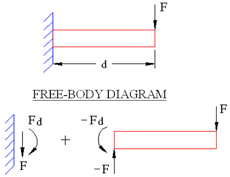
Figure 1: Free-Body Diagram of a Cantilever Beam
F = Reaction force exerted on wall by beam.
Fd = Reaction moment exerted on wall by beam.
The internal force calculator reports reactions at all nodes in the model. This can be enabled by activating the Calculate reaction forces check box in the Solution tab of the Analysis Parameters dialog box. Typically, only nodes with some boundary condition give nonzero reactions. The internal force calculator produces a filename.ro file. The .ro file is a direct access unformatted file containing nodal reactions, nodal applied forces and their difference at nodes. This file is just like the .do file and can be used in the Results environment (of course there are three times the number of load cases). The text results of the reaction forces are written to the filename.l file.
The structural analysis solves the following equation system:
K D = F (Kij Dj = Fi j sum)
where
K is the stiffness matrix
D is the vector of nodal displacements/rotations
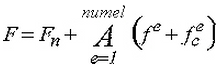
F is the vector of applied loads and boundary conditions
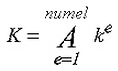
A is the assembly operator
k e is the element level stiffness matrix
f e is the element level applied force vector (includes tractions, body forces, thermal loads, and so on)
![]() is the element level vector of applied centrifugal forces
is the element level vector of applied centrifugal forces
d e is defined as the element displacement vector (i.e. from vector D pull out values corresponding to element nodes)
F n is the vector of nodally applied forces/moments
The internal force calculator uses the following definitions:
R = -KD = nodal reaction
F = applied nodal forces
F - KD = nodal residual (R + F)
-k e d e = element reaction
f
e
+![]() = element applied force
= element applied force
The structural analysis computes centrifugal forces as nodal forces rather than as element level body forces. Boundary, gap and rigid elements do not have mass and hence do not contribute to centrifugal loading.
For the reaction forces to be computed correctly, the processor must be consistent; i.e. the element routines should be the same for internal forces processor and the linear stress processor. An out-of-sync processor gives rise to nonzero residuals at unrestrained nodes. Beware of situations where rectangular elements give zero residuals while distorted elements do not - this could be a synchronization issue.
Sometimes it is convenient to ignore some elements for the reaction computations (e.g., to find the reaction on nodes attached to a boundary element, the boundary element stiffness should not be assembled to K). This can be done by pressing the Settings button. The resulting dialog box has a table where the first column states the part number, the second column states a description that you can add and the third column provides the following options when you click in it:
Loads and Elements
- Output the reaction forces for all nodes and elements in this part.
-
Elements Only
Output only the reaction forces for the elements. -
Ignore
The elements and nodes of this part is ignored when reaction forces are computed.
If you have boundary elements in your model (1D springs, 3D springs, or prescribed displacements), you must activate the Ignore boundary element groups check box to get accurate results for the reaction forces. This causes the processor to not calculate the reaction forces for the boundary elements, which would cancel out the opposite reaction forces at the model nodes to which the boundary elements are attached. The Ignore boundary element groups option is activated by default.
Solver Options
The type of solver for a static stress analysis can be selected in the Type of solver drop-down Menu in the Solution tab of the Analysis Parameters dialog box. See also Types of Solvers Available for background information. The options available are as follows:
- Automatic: This is the default option. If selected, the processor chooses between the Iterative (AMG) and Sparse options based on the model size (that is, on the number of degrees of freedom to solve). The sparse solver is typically optimum for small to mid-sized models. The iterative solver is generally optimum for large models, and it requires less RAM.
- Sparse: Uses one of the sparse solvers available in the Type of sparse solver drop-down menu. The sparse solvers use multiple threads/cores when available (see the Sparse Solver Section topic below).
- Iterative (AMG): Uses the Algebraic Multi-Grid iterative scheme to solve the system of equations. This solver uses multiple threads/cores when available. It is the default for models with a large number of degrees of freedom to solve and is recommended for models with thin walls, slender parts, plate/shell or beam elements, multipoint constraints (MPCs), and for ill-conditioned models.
- Iterative (AMG-MF): This is a variant of the Iterative (AMG) solver, adapted from Autodesk Moldflow technology. It is best suited for models with relatively thick or fat part volumes and may provide a performance advantage, relative to the Iterative (AMG) solver, for such models. You must manually select this solver; the Automatic option will only use the Iterative (AMG) solver for large models. The Iterative (AMG-MF) solver uses multiple threads/cores when available.
When the Iterative (AMG-MF) solver is selected, an additional option becomes available within the Solution tab of the Analysis Parameters dialog box. Specifically, this solver can take advantage of GPU (Graphics Processing Unit) computing, in which the many small cores of the GPU assist with the computation-intensive task. Activate the option, Use the GPU version of the solver, to take advantage of this capability.
If for some reason you want to create the stiffness matrix but not perform the analysis, activate the check box for Stop after stiffness calculations. The only time this is useful is if you are using the stiffness matrix for other purposes, such as accessing it from another program. The stiffness matrix is always calculated when running an analysis, so there is no advantage to use this option in normal circumstances.
For the sparse and iterative solvers, the Percent memory allocation field controls how much of the available RAM is used to read the element data and to assemble the matrices. A small value is recommended. (When the value is less than or equal to 100%, the available physical memory is used. When the value of this input is greater than 100%, the memory allocation uses available physical and virtual memory.)
As listed above, some of the solvers take advantage of multiple threads/cores available on the computer. The drop-down Number of threads/cores control is enabled in such situations. You want to use all the threads/cores available for the fastest solution, but might choose to use fewer threads/cores if you need some computing power to run other applications at the same time as the analysis.
Iterative Solver Section
If the iterative solver is chosen, then the Iterative Solver section is enabled. The input for this section is as follows:
- The Convergence tolerance field determines how accurate of a solution to the matrix of equations is found. The smaller the tolerance, the more accurate the solution.
- Maximum number of iterations stops the analysis if the matrix of equations is not solved within this number of iterations.
- The accuracy of the solution depends on the convergence tolerance; a smaller tolerance results in a more accurate solution but may take more iterations. As with any iterative solution, the results should be checked to confirm that they meet the appropriate accuracy. In some cases, performing the analysis twice with a different convergence tolerance is the best way to confirm the accuracy.
- For static stress analysis, one check on the accuracy is the reaction forces. The end of the summary file (viewable from the browser in Report environment or by editing the summary file with Notepad) includes a summary of the reaction forces and other parameters. A large unfixed direction residual can indicate a poorly converged solution. Naturally, you can also check in the Results environment whether the sum of the residual forces (the support reactions) matches the applied loads.
Sparse Solver Section
If the sparse solver is chosen, then the Sparse Solver section is enabled. The input for this section is as follows:
- The Type of sparse solver drop-down menu contains the sparse solvers currently available. If you choose a solver that is not available on an operating system, the processor uses the best one for the operating system. For example, if MUMPS is set (available only for Linux) and you run the model on Windows, the BCSLIB-EXT solver is used instead. The sparse solvers available are as follows:
-
- Default: use BCSLIB-EXT.
- BCSLIB-EXT: (Windows and Linux) use the Boeing solver. For Windows only, the BCSLIB-EXT solver may write temporary files to the folder specified by the environment variable USERPROFILE. By default, this variable is set to the folder C:\Documents and Settings\Username where C: is the drive on which the operating system is installed. The error numbers -701 or -804 returned from the BCSLIB-EXT solver means that it ran out of hard disk space for storing the temporary files. If this occurs, change the USERPROFILE variable to a directory that can provide sufficient hard disk space. (See the Windows Help and Support for documentation on changing environment variables.)
- MUMPS: use the MUMPS distributed solver. Note:
- The distributed solver requires MPI to be installed on the computers. Refer to the MPICH2 on Windows page or the MPI Clusters on Linux page within the Simulation Mechanical Supplement of the Autodesk Installation and Licensing Guide for details.
- The MUMPS distributed solver cannot be used on Windows when the analysis includes gap or contact elements.
- The Solver memory allocation field sets the amount of memory to use during the sparse matrix solution for the BCSLIB-EXT solver. In general, allocating more memory should result in a faster analysis. The other sparse solvers adjust the memory setting automatically; so no setting is required for them.
Contact Options
Surface Contact
If you are performing an analysis with contact, there are three methods that can be used during the iterative process in which it is determined which nodes are in contact. This can be specified in the Iteration method drop-down menu in the Contact tab of the Analysis Parameters dialog box. The Individual points option is the most conservative approach; it activates/deactivates each point, and only considers multiple points simultaneously if all have identical states. This method is suggested for hand-built models employing gap elements. The Mixed option simultaneously activates all inactive contact points in compression but deactivates those not in compression, one at a time. The Multiple option is the most aggressive, as it activates or deactivates all gaps requiring a change in state. This last option, can lead to unstable solutions, but, when stable, can result in the most expedient solution. All three methods are applicable to surface and edge contact, with the latter two being suggested.
The nonlinear structural analysis associated with contact is linearized into many piecewise linear calculation steps. This process is continued until equilibrium is reached or until the number of iterations exceeds the value specified in the Maximum number of iterations dialog box.
The Threshold tolerance field is used to prevent unwanted oscillatory behavior during contact. Contact elements with an absolute strain below this (small) value do not change state from one iteration to the next. Thus, elements which would otherwise have their state changed from enabled to disabled, or vice versa, remain in their current state during this particular iteration. A typical value for this entry is usually less than 0.01.
Many contact problems result in unstable solutions for the first iteration. Furthermore, if rigid-body motion is possible, then unstable solutions occur for all iterations. This is purely an artifact that the underlying mathematics results in singular or in very ill-conditioned systems when structures are not affixed. To prevent such solution problems, a stabilization method is usually employed. Three different options are available in the Stabilization method drop-down menu. all these stabilization options pre-activate all contact points for the first iteration. The Global/Initial option utilizes the same small value for the stiffness throughout the model, and is only applied prior to the first iteration. Thus, it is particularly well suited for models not exhibiting rigid-body motion. The other two options are not only applied prior to the first iteration, but simulated constraints are added for all iterations to prevent rigid-body motion. These options employ artificial stiffness to enforce this constraint. The Local option requires you to specify a number used to establish this stiffness. The input number is the ratio of this stiffness relative to the largest stiffness present in the structural model. This number should lie between 0 and 1. There is also the option to avoid using a stabilization method.
If the Local option is selected, you are required to specify a value that is used to establish this stiffness. This is done in the Stabilization factor field. The input number is the ratio of this stiffness relative to the largest stiffness present in the structural model. This number should be between 0 and 1.
If a solution has not converged when the maximum number of iterations is reached, the contact stiffness can be reduced by a factor of 10. It happens as many times as specified in the Stiffness reduction attempts drop-down menu.
Bonded Contact
There are two methods of handling bonded connections. Which method is used depends in part on whether the nodes are matched between the two parts or not matched.
Activating the option Enable smart bonded/welded contact uses multi-point constraint equations (MPCs) when necessary to bond the nodes on part A, surface B with the nearest nodes on part C, surface D. Shape functions interpolate the displacements at the nodes on surface B to the nodes on surface D. Therefore, the meshes do not need to match between the parts. The MPCs are used for all the nodes on the surface contact pair whenever any node does not match. If the meshes do match at all nodes, then node matching is used to bond the contact surface; the two vertices on the adjoining parts are collapsed to one node, and MPC equations are not used for the contacting surfaces. The options for the smart bonding drop-down are as follows:
- None Smart bonding is not used. Therefore, the nodes must match for parts to be bonded.
- Coarse bonded to fine mesh Smart bonding creates MPC equations that connect the nodes on the surface with the coarser mesh to the nodes on the surface with the finer mesh.
- Fine bonded to coarse mesh Smart bonding creates MPC equations that connect the nodes on the surface with the finer mesh to the nodes on the surface with the coarser mesh.
The smart bonding option applies to bonded contact and welded contact. Other types of contact (except for Free) require the nodes to be matched. See the page Meshing Overview: Creating Contact Pairs: Types of Contact for a discussion of defining contact and additional information about using smart bonding.
By default, smart bonding uses the condensation method to solve your analysis. If you find your analysis doesn't converge or is not performing as you expect, you can try a different Solution method to use with MPC equations (see Multi-Point Constraints). Click SetupLoadsMulti-Point Constraint and choose from the Solution method options. If you use the Penalty Method, the accuracy of the solution is controlled by the Penalty multiplier field. The Penalty multiplier, times the maximum diagonal stiffness in the model, is used during the penalty solution. A value in the range of 10
4
to 10
6
is recommended.
- The solution method you select in the Define Multi-Point Constraints dialog box becomes the method used for all features that include MPCs. These features include, but are not limited to, cyclic symmetry, frictionless constraints, smart bonding, and user-defined MPCs. For example, if you want to use the Penalty Method to solve all your analyses involving smart bonding, you can override the default condensation method by selecting Penalty Method in the Define Multi-Point Constraints dialog box.
- Smart bonding applied to contact between brick, 2D, membrane, and plate elements. Bonded contact involving other element types requires the nodes to match and are not affected by the smart bonding setting.
When the option Enable smart bonded/welded contact is not activated, the parts are bonded only if the nodes match between the parts.
Control Data in Output Files
Before performing the analysis, you can select additional output to be created. The Output tab of the Analysis Parameters dialog box can be used to control what data is output. all the output goes to various text files except for the following:
- Stress/strain at midside nodes (binary) If activated, the stress and strain at midside nodes is output to the binary result files. These results can then be displayed in the Results environment. (Midside nodes are an option that can be activated for certain element types using the Element Definition dialog box.)