Brick elements are 8- to 21-node isoparametric or sub-parametric curvilinear hexahedra. Typical elements are illustrated in Figure 1. These elements may be used to model 3D solids or thick shells, such as the two examples in Figure 2.
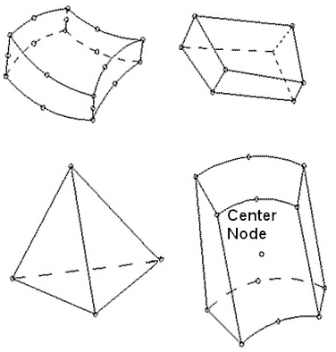
Figure 1: Typical 3D Continuum Elements Derived from the General 21-Node Element
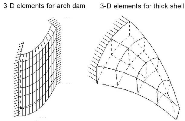
Figure 2: Typical Applications for 3D Elements
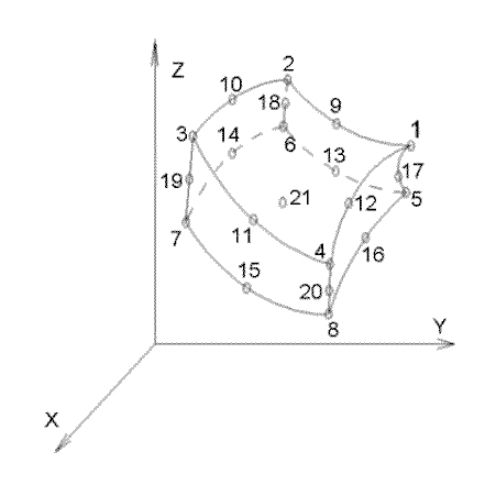
Figure 3: Sample 3D Brick Model
Three-dimensional solid elements are Type 25 elements. A general 3D isoparametric element with a variable number of nodes from 8 to 21 can be used. The first 8 nodes are the corner nodes of the element; nodes 9 to 20 correspond to mid-side-nodes and node 21 is a center node. The element can be used for 3D analysis of solids and thick shells. As with the 2D elements, the possibility of choosing different element node configurations allows effective finite element modeling.
Determination of Surface Numbers for Eight-Node Bricks
When applying loads to a surface number of a brick part, be aware that some models may not have all the lines on the face to be loaded on the same surface number. What happens in this situation? If the model originated from a CAD solid model, all faces coincident with the surface of the CAD model will receive the load regardless of the surface number of the lines. In hand-built models and on CAD parts that are altered so that the part is no longer associated with the CAD part, the surface number that is common in any three of the four lines that define a face (four-node region) or two of the three lines (three-node region) determines the surface number of that face.
Brick Element Parameters
First, you must specify the material model for this part in the Material Model list box under the Element Definition dialog. The available brick material models are grouped in the following categories. Refer to the appropriate page under the Material Properties page for details on each of the material models.
-
Elastic
- Isotropic: This material model option is used for parts that will only experience deflections in the elastic region of the stress-strain curve. To use this material model, the parts must have identical material properties in all directions. A single modulus of elasticity and Poisson's ratio will be the requested material properties.
- Orthotropic: This material model option is used for parts that will only experience deflections in the elastic region of the stress-strain curve. The part may have different material properties in certain directions. Specifically, the material properties may be different in one or more of the three orthogonal directions in a rectangular coordinate system.
- Curve: This material model option is also used for the analysis of geological materials. In this model, the instantaneous bulk and shear moduli are defined by piece-wise linear functions of the current volume strain.
- Thermoelastic: This material model is used to model materials what will only experience deflections in the elastic region of the stress-strain curve but may also experience stress due to a temperature difference.
- Temperature Dependent Orthotropic: This material model is used for parts that have different material properties in certain directions that also vary with the temperature. Specifically, the material properties may be different in one or more of the three orthogonal directions in a rectangular coordinate system. The material properties will be specified at multiple temperatures. The values will be linearly interpolated between temperature values. The temperature range for which the material properties are defined must include the expected temperatures.
- Duncan-Chang Soil: The Duncan-Chang (1970) model is used to simulate soil. It is based on tri-axial soil tests and assumes a hyperbolic stress-strain relation. When using this material model, the Analysis Formulation on the Advanced tab is set to Material Nonlinear Only.
- Moldflow: If the part is injection molded, the anisotropic material properties that result from the molding process can be obtained from an Autodesk Moldflow simulation. Select Moldflow as material model. See Interoperability with Autodesk® Simulation Moldflow® for details.
-
Hyperelastic
Tip: Using a higher integration order (set on the Advanced tab) for hyperelastic and foam materials can help with convergence when the part experiences large deformation.
- Mooney-Rivlin: This material model is used to model hyperelastic materials such as rubber.
- Arruda-Boyce: This material model is a hyperelastic material model used to model rubber materials. The implementation follows the Ogden material behavior for volume-preserving deformation modes.
- Ogden: This material model is used to model hyperelastic materials such as rubber.
- Yeoh: This material model is used to model nearly incompressible (volume preserving) hyperelastic materials, such as rubber. Only Total Lagrangian analysis formulation is available.
- Neo-Hookean: This material model is used to model nearly incompressible (volume preserving) hyperelastic materials, such as rubber. Only Total Lagrangian analysis formulation is available.
- Van der Waals: This material model is used to model nearly incompressible (volume preserving) hyperelastic materials, such as rubber. Only Total Lagrangian analysis formulation is available.
-
Foam
- Blatz-Ko: This material model involves strong coupling between volumetric and non-volumetric parts, such as the bulk modulus, cannot be determined separately as with other hyperelastic material models.
- Hyperfoam: This material model is used to hyperelastic materials similar to the Ogden material model. This material model will account for the compressibility of the material. This is not applicable to plane strain elements.
-
Viscoelastic
- Viscoelastic Arruda-Boyce: A viscoelastic variation of the Arruda-Boyce (hyperelastic) material model.
- Viscoelastic Blatz-Ko: A viscoelastic variation of the Blatz-Ko (hyperfoam) material model.
- Thermal Creep Viscoelastic: This material model is used to model materials that will only experience deflections in the elastic region of the stress-strain curve but may also experience creep. Creep occurs when a model deflects under a constant load over time. See the paragraph Defining Thermal Properties of Brick Elements for setting up the creep law to use with this material model.
- Viscoelastic Ogden: A viscoelastic variation of the Ogden (hyperelastic) material model.
- Viscoelastic Hyperfoam: A viscoelastic variation of the Hyperfoam material model.
- Linear Viscoelastic Isotropic: This is a viscoelastic material model in which the material exhibits properties of an elastic solid and a viscous fluid. The viscoelastic properties are based on the Prony series. The properties are equal in all directions (isotropic) and independent of temperature.
- Linear Viscoelastic Orthotropic: This is a viscoelastic material model in which the material exhibits properties of an elastic solid and a viscous fluid. The viscoelastic properties are based on the Prony series. The properties are different in three perpendicular directions (orthotropic) and independent of temperature.
- Linear Thermal Viscoelastic Isotropic: This is a viscoelastic material model in which the material exhibits properties of an elastic solid and a viscous fluid. The viscoelastic properties are based on the Prony series. The properties are equal in all directions (isotropic) and dependent on temperature.
- Linear Thermal Viscoelastic Orthotropic: This is a viscoelastic material model in which the material exhibits properties of an elastic solid and a viscous fluid. The viscoelastic properties are based on the Prony series. The properties are different in three perpendicular directions (orthotropic) and dependent on temperature.
- Viscoelastic Mooney-Rivlin: A viscoelastic variation of the Mooney-Rivlin (hyperelastic) material model.
- Viscoelastic Neo-Hookean: A finite strain, viscoelastic variation of the Neo-Hookean (hyperelastic) material model.
- Viscoelastic Yeoh: A finite strain, viscoelastic variation of the Yeoh (hyperelastic) material model.
- Viscoelastic Van der Waals: A finite strain, viscoelastic variation of the Van der Waals (hyperelastic) material model.
-
Plastic
- von Mises with Isotropic Hardening: This material model option is used for parts that may experience plastic deformation during the analysis. A bilinear curve will be defined to control the stress-strain relationship.
- von Mises with Kinematic Hardening: This material model option is also used for parts that may experience plastic deformation during the analysis. A bilinear curve will be defined to control the stress-strain relationship. This material model option is preferred over the von Mises with Isotropic Hardening material model option if the model will undergo cyclical loading.
- von Mises Curve with Isotropic Hardening: This material model option is used for parts that may experience plastic deformation during the analysis. You will be able to specify a stress-strain curve with multiple data points to control the stress-strain relationship.
- von Mises Curve with Kinematic Hardening: This material model option is used for parts that may experience plastic deformation during the analysis. You will be able to specify a stress-strain curve with multiple data points to control the stress-strain relationship. This material model option is preferred over the von Mises with Isotropic Hardening material model option if the model will undergo cyclical loading (Bauschinger effects).
- Thermoplastic: This material model is used to model materials what may experience plastic deformation during the analysis and may also experience stress due to a temperature difference.
-
Viscoplastic
- Thermal Creep Viscoplastic: This material model is used to model materials that may experience plastic deformation and may also experience creep. Creep occurs when a model deflects under a constant load over time. See the paragraph Defining Thermal Properties of Brick Elements for setting up the creep law to use with this material model.
- Drucker-Prager: This material model is similar to the von Mises material models but has the addition of a yielding function. The model assumes that the volumetric strain changes the yielding function. This occurs in materials such as concrete and rock.
-
Concrete
- Reinforced Concrete: This material model allows different tensile and compressive behaviors. It can simulate cracking and crushing failure of concrete under relatively monotonic loading. Cracking and crushing are simulated via degeneration of the elasticity at the integration points instead of tracking individual macroscopic cracks. A maximum of three independent directions of rebars are allowed for the concrete material. However, the details of the rebar locations (in height or depth) are not considered; they are treated as smeared throughout the part. If using the reinforced concrete material model, the Analysis Formulation on the Advanced tab will be set to Material Nonlinear Only.
-
Electrical
- Piezoelectric: This material model is used for parts that will experience stress as a result of a voltage difference. You will need to supply both the elastic and piezoelectric properties.
- General Piezoelectric: This material model is a generalized form of the Piezoelectric material model. You will need to supply the elastic stiffness and piezoelectric matrices coefficients.
For the brick elements in this part to have the midside nodes activated, select the Included option in the Midside Nodes drop-down box. If this option is selected, the brick elements will have additional nodes defined at the midpoints of each edge. (For meshes of CAD solid models, the midside nodes follow the original curvature of the CAD surface, depending on the option selected before creating the mesh. For hand-built models and CAD model meshes that are altered, the midside node is located at the midpoint between the corner nodes.) This will change an 8-node brick element into a 20-node brick element. An element with midside nodes will result in more accurately calculated gradients. This is especially useful when trying to model bending behavior with few elements across the bending plane. Elements with midside nodes increase processing time. If the mesh is sufficiently small, then midside nodes may not provide any significant increase in accuracy.
Use the Analysis Type drop-down to set the type of displacement that is expected. Small Displacement is appropriate for parts that experience no motion and only small strains and will ignore nonlinear geometric effects that result from large deformation. (It also sets the Analysis Formulation on the Advanced tab to Material Nonlinear Only.) Large Displacement is appropriate for parts that experience motion and/or large strains. (The Analysis Formulation on the Advanced tab should also be set as required for the analysis.)
When you use a Moldflow material model, use the Residual Stress (Moldflow Insight Only) drop-down to include or exclude residual stresses for your analysis. If set to Include, stresses built-up during the injection molding process are modeled. Upon ejection from the mold, the part shrinks and warps to redistribute the stresses incurred while in the mold. Your model part represents the in-mold dimensions.
- The displacement at midside nodes is always output. The stress and strain at midside nodes are output only if the user activates the option to output these results before running the analysis. The option is located under the Setup
 Model SetupParametersAdvanced dialog on the Output tab. (See the page Setting Up and Performing the Analysis: Nonlinear: Analysis Parameters: Advanced Settings: Controlling the Output Files for details.)
 - Use the
 Options Analysis tab and set the Use large displacement as default for nonlinear analyses option to control whether the Analysis Type defaults to small or large displacement.
Define Thermal Properties of Brick Elements
Thermal Section:
If a brick element part is using a material model that includes thermal effects, you must specify a value in the Stress free reference temperature field in the Thermal tab of the Element Definition dialog. This value is used as the reference temperature to calculate element-based loads associated with constraint of thermal growth using bilinear interpolation of the nodal temperatures.
Creep Section:
If a brick element part is using a material model that includes creep, select the option in the Creep law drop-down box. This selection will be used to calculate the creep effects during the analysis. The creep laws available are as follows:
- No creep: When this option is chosen, no creep effects are included in the analysis.
- Power-law: This option is also known as the uniaxial creep law. The equation is
 = C
1
x
= C
1
x C2
x t
C3
.
C2
x t
C3
. - Garofalo: This option is also known as the hyperbolic sine creep law. The equation is = A
0
x [sinh(A
1
x )]
A2
.
- Double power-law: This option is similar to the power law but with an additional term to produce results closer to experimental results at high stress levels. The equation is = C
1
x
C
2
x t
C3
+ C
4
x
C5
x t
C6
.
where![]() is the effective creep strain rate and
is the effective creep strain rate and![]() is the effect stress. Also refer to the page Setting Up and Performing the Analysis: Nonlinear: Material Properties: Thermal Creep Viscoelastic Material Properties for important information on entering the material properties.
is the effect stress. Also refer to the page Setting Up and Performing the Analysis: Nonlinear: Material Properties: Thermal Creep Viscoelastic Material Properties for important information on entering the material properties.
For the creep calculations to be calculated on evenly sized divisions of the time step, select the Fixed substeps option in the Time integration method drop-down box. For the creep calculations to be calculated on variable sized divisions of the time step, select the Flexible substeps option. These two methods are based on time hardening and use explicit time integration methods. These methods may become unstable under some loading conditions. When using the Thermal Creep Viscoelastic material model and the Creep strain definition drop-down box is not set to Modified, an additional option will be available in the Time integration method drop-down box: the Alpha-method. This method uses an implicit time integration scheme to improve the creep behavior. This method can be unconditionally stable.
Specify the temperature at which no thermal stress exists in the Stress free reference temperature field.
If you are performing an analysis with non-cyclical loading, select the Effective option in the Creep strain definition drop-down box. If you are performing an analysis with cyclical loading, select the Modified option.
During the analysis, the creep calculations will be performed as iterations in substeps of each time step. You can control how many substeps are allowed in a single time step in the Maximum number of substeps field. You can also specify how many iterations can be performed in a single substep in the Maximum number of iterations in a substep field. After each substep iteration, the creep stress and strain will be compared to the previous iteration. If the value is not within the tolerances specified in the Creep strain calculation tolerance and Creep stress calculation tolerance fields, another iteration will be required.
When using a Time integration method of Alpha-method, the Time integration parameter needs to be specified. To use a fully explicit method for the time-integration scheme (but different than the fixed/flexible substeps' explicit method), type 0.0 in the Time integration parameter field. To use a fully implicit method, type 1.0 in the Time integration parameter field. When the Time integration parameter is greater than 0.5, this method is unconditionally stable.
Control Orientation of Brick Elements
If this part of brick elements is using an orthotropic or general piezoelectric material model, you will need to define the orientation of material axes 1, 2 and 3 in the Orthotropic or Aniostropic tab of the Element Definition dialog, respectively. There are two basic methods to accomplish this.
Method 1:
The first method is to select one of the global axes as material axis 1. If you select the Global X-direction option in the Material axis direction specified using drop-down box, the orthogonal material axes follow the X, Y and Z axes as follows:
- Material axis 1: X axis
- Material axis 2: Y axis
- Material axis 3: Z axis
If you select the Global Y-direction option in the Material axis direction specified using drop-down box, the orthogonal material axes follow the X, Y and Z axes as follows:
- Material axis 1: Y axis
- Material axis 2: Z axis
- Material axis 3: X axis
If you select the Global Z-direction option in the Material axis direction specified using drop-down box, the orthogonal material axes follow the X, Y and Z axes as follows:
- Material axis 1: Z axis
- Material axis 2: X axis
- Material axis 3: Y axis
With the first method, the axes can be rotated about the chosen global direction by entering an angle in the Material Axis Rotation Angle field. This angle follows the right-hand rule.
Method 2:
The second method is to select the Spatial Points option in the Material axis direction specified using drop-down menu. Next you must define the coordinates for three spatial points in the Spatial point coordinates table. Next, select the appropriate index for the spatial points in the Index of spatial point 1, Index of spatial point 2, and Index of spatial point 3 drop-down menus.
- Material axis 1 is a vector from the spatial point in the Index of spatial point 1 drop-down menu to the spatial point in the Index of spatial point 2 drop-down menu.
- Material axis 2 is perpendicular to local axis 1, lies in the plane formed by the three spatial points, and is on the same side of axis 1 as the spatial point in the Index of spatial point 3 drop-down menu.
- Material axis 3 is calculated as the cross-product of material axes 1 and 2.
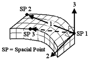
Figure 4: Orientation of Material Axes
Advanced Brick Element Parameters
Analysis Formulation:
Select the formulation method that you want to use for the brick elements in the Analysis Formulation drop-down box in the Advanced tab.
- If the Material Nonlinear Only option is selected, nonlinear material model effects will be accounted for but all calculations will be performed based on the undeformed geometry. Thus, this formulation is suitable for parts with small strains and no motion. This will be the only option available if the Analysis Type on the General tab is set to Small Displacement.
- The Total Lagrangian option will refer to the initial undeformed configuration of the model for all static and kinematic variables. This formulation is suitable for parts with motion and small strains. Note that the material properties should be in terms of engineering stress and strain.
- The Updated Lagrangian will refer to the last calculated configuration of the model for all static and kinematic variables. This formulation is suitable for parts with motion and large strain. Note that the material properties should be in terms of actual stress and strain.
Compatibility:
Select whether you want the compatibility to be Enforced or Not Enforced in the Compatibility drop-down box. If the Not Enforced option is selected, gaps or overlaps are allowed along interelement boundaries. These elements are formulated using an assumed linear stress field. These elements are most effective as low aspect ratio rectangles. With this option selected, the elements are formulated using an assumed linear stress field. If the Enforced 'option is selected, openings, overlaps or discontinuities are not allowed along interelement boundaries. These elements are formulated using an assumed linear displacement field. These elements can overestimate the stiffness of the structure. In general, a greater mesh density in the direction of the strain gradient is required to achieve the same level of accuracy as elements for which the Not Enforced option is selected. With this option selected, the elements are formulated using an assumed linear displacement field.
Stress Update Method:
The Stress Update Method is used when the material model (on the General tab) is set to one of the following plastic material models:
- von Mises with Isotropic Hardening
- von Mises with Kinematic Hardening
- von Mises curve with Isotropic Hardening
- von Mises curve with Isotropic Hardening
This controls the numerical algorithm for integrating the constitutive equations (stress/strain law) when the material goes plastic. The options available for the Stress Update Method are as follows:
- Explicit: (Original method). This option uses the explicit sub-incremental forward-Euler method for integrating the constitutive equations. The Explicit option is best used for simple problems, such as simple tension, because the method runs faster. However, it is more sensitive to the loading, time step size, and complexity of the material stress-strain curve.
- Generalized Mid-Point: This option uses an implicit method for integrating the constitutive equations. It reduces the error accumulation and can ensure that the stress updating process is unconditionally stable. Thus, this option is better suited for complicated analyses, such as contact problems, severe plasticity, or complex material stress-strain curves.
Stress Update Method Guidelines:
- Verify that the analysis results make sense (that is, that they follow the expected behavior). For example, if there is symmetry in the geometry, loads, and boundary conditions, symmetrical results are expected (except for anisotropic materials). If the results are counterintuitive or if there are discontinuities or instability in the solution, change the Stress Update Method or increase the updating rate of the variables, as discussed in the next guideline.
- Whether you choose Explicit or Generalized Mid-Point, more frequent updating of the stress and strain variables improves the solution for plastic material models. Use one of the following methods to increase the updating rate:
- Reduce the time step size (increase capture rate) in the Analysis Parameters.
- Instead of Automatic or Combined Newton, choose the Full Newton option for the Nonlinear iterative solution method in the Equilibrium tab of the Analysis Parameters - Advanced dialog box.
- The Generalized Mid-Point method is typically able to tolerate larger time steps than the Explicit method – while obtaining more accurate results – but it is computationally more expensive.
- Background: Integrating the constitutive relations to obtain unknown stress increments is crucial to mechanical event simulation (MES). These relations define a set of ordinary differential equations, and methods for integrating them are usually classified as explicit or implicit. The explicit method only looks forward. That is, the slope of the material stress-strain curve is chosen at the beginning of an increment, and this slope is used to calculate stress at the end of the increment. For the implicit method, the solver looks forwards and backwards, and the slope has to be calculated using multiple iterations. The strain increment is multiplied by the slope of the stress-strain curve to determine the stress.
In the Explicit integration scheme, the yield surface, plastic potential gradients, and hardening law are all evaluated at known stress states. No particular iteration is strictly necessary to predict the final stresses.
In the Generalized Mid-Point scheme (which is a type of implicit method), simple iterative adjustment restores the next increment's stresses and hardening parameters to the yield surface, since this condition is not enforced by the integration. This correction requires additional effort for solving the nonlinear equations iteratively. Conversely, explicit methods do not require the solution of a system of nonlinear equations to compute the stresses at each Gauss point.
The Parameter for Generalized Mid-point input is used when the Stress Update Method is set to Generalized Mid-Point. Acceptable ranges for this input are 0 to 1, inclusive. When the Parameter is set equal to 0, the resulting algorithm would be a fully explicit member of the algorithm family (similar to the Explicit option for the Stress Update Method); however, the solution is not unconditionally stable. When the Parameter is 0.5 or larger, the method is unconditionally stable. When the Parameter is set to 0.5, the solution is known as a mid-point algorithm; when it is 1, the solution is known as the fully backward Euler or closest point algorithm and is fully implicit. A value of 1 is more accurate than other values, especially for large time steps.
Strain Measurements:
The Strain Measurements is used when the Material Model (on the General tab) is set to Isotropic and the Analysis Formulation is set to Updated Lagrangian. The options are used to improve the convergence of the updated Lagrangian method. The options available for the Strain Measurements are as follows:
- Almansi Strain: (Original method). This option uses the Cauchy stress and Almansi strain for the constitutive relation. It is limited to cases of small strain.
- Log-strain: This option uses the Cauchy stress and virtual log-strain (incremental strain) for the constitutive relation. It is acceptable for all cases, including large strain. This is a hypoelastic model, and one drawback is that it works better for incompressible material (Poisson ratio = 0.5) than compressible materials. This is because the shear modulus is assumed to be a constant where as it changes with the varying volume in reality.
Integration Order:
Select the integration order that will be used in this part using the 1st Integration Order and 2nd Integration Order drop-down boxes. The 1st integration order setting controls integrations in the global X and Y directions. The 2nd integration order setting controls integrations in the Z direction.
Automatically meshed solids will typically have elements with comparable lengths in the three global directions and may have comparable stress gradients in all directions. In such cases, set both integration order inputs to the same order. Situations where you may want to use a different integration order in the Z direction include the following:
- The stress gradient in the model is significantly greater or lesser in the Z direction than in the other two directions.
- The mesh is hand-built with the element length in the Z direction compressed or elongated relative to the X and Y directions.
- For rectangular shaped elements, select the 2nd Order option.
- For moderately distorted elements, select the 3rd Order option.
- For extremely distorted elements, select the 4th Order option.
The computation time for element stiffness formulation increases as the third power of the integration order. Consequently, the lowest integration order that produces acceptable results should be used to reduce processing time.
Overlapping Elements:
If the Allow for overlapping elements check box is activated, overlapping elements will be allowed to be created when the lines are decoded into elements. Overlapping may be necessary when modeling elements. This is especially true for problems confined to planar motion.
Output Options:
For the stress results for each element to be written to the text log file at each time step during the analysis, activate the Detailed force and moment output check box. This may result in large amounts of output data.
If one of the von Mises material models has been selected, you can choose to have the current material state (elastic or plastic), current yield stress limit, current equivalent stress limit and equivalent plastic strain output at corner nodes and/or integration points at every time step. This is done by selecting the appropriate option in the Additional output drop-down box.
Selective Reduced Integration (Mean-dilatation):
Many physical problems involve motions that essentially preserve volumes. Materials that behave in this fashion are termed incompressible. For example, rubber and metals with rigid-plastic flow are nearly incompressible. Activating the Selective Reduced Integration (Mean-dilatation) check box will add a modification to the usual compressible FEA formulations that represents the incompressible limit and high-compressible volume change. This method (B-Bar) helps avoid the volumetric locking.
When not activated (unchecked), the dilatational components of deformations (volume related) are integrated at the same order with the deviatoric components. When activated (checked), the mean value is used to compute the dilatational contribution.
Two examples in which this option will benefit the analysis are as follows:
- Material Properties: In isotropic linear elasticity, the condition of incompressibility may be expressed in terms of Poisson's ratio. As the Poisson ratio approaches 0.5, resistance to volume change is greatly increased - assuming resistance to shearing remains constant. In another word, the bulk modulus approaches infinity.
- Material Models and Deformation: In elasto-plastic material models, the plastic deformation is much larger than the elastic deformation, and mechanical theory assumes there is no volume change in plastic deformation. Thus, the material is practically constant volume. Similar assumptions also exist in other nonlinear material models.
Piezoelectric Material Options:
When one of the piezoelectric material models has been chosen for a part, two additional options will become available within the Advanced tab of the Element Definition dialog box...
- Use the Nodal voltage load curve input field to specify the number of the load curve that will be used to control all nodal voltages throughout the analysis event.
- Voltage differentials applied across piezoelectric materials produce an electrical field that causes the piezoelectric part to deform slightly. The amount of strain is typically small. The deformation of the part has a small effect on the electrical field, which in turn has a slight effect on the resultant piezoelectric deformation. To take this effect into account, activate the Update electric field checkbox. Otherwise, the electrical field will be based on the initial (undisplaced) condition of the part.
Define Soil Conditions
If the Duncan-Chang material model is chosen, the Soil tab is enabled. Enter the following input as appropriate for the analysis. This input is related to the initial state of the soil; also see the page Setting Up and Performing the Analysis: Nonlinear: Material Properties: Duncan-Chang Material Properties: Duncan-Chang Theoretical Description for information.
- Superimpose hydrostatic pressure When activated, the initial stress is created from a constant hydrostatic pressure entered in the accompanying field. (Hydrostatic pressure in this case is acting equally in all directions, not to be confused with a pressure that increases with depth) The magnitude of the pressure must be greater than 0.
- Superimpose self weight When activated, the initial stress is created from the weight of the modeled soil.
- Reference point on surface Specify an X, Y, Z coordinate. This establishes where the pressure due to the weight of the soil is zero. If the model is a section of soil deep underground, then the reference point can be above the part modeled.
- Coefficient of lateral earth pressure Most soils do not create a true hydrostatic stress (equal in all directions). The stress in the horizontal directions is normally some fraction of the vertical normal stress. The ratio of lateral/vertical stress defines the coefficient of lateral earth pressure. The input should be in the range of 0 to 1.
- Gravitational acceleration To create a stress distribution due to the self weight, enter the gravitational constant and direction in which gravity was acting to create the stress distribution. The direction is normally the same direction that gravity acts in the analysis. However, a different direction can be used if the model represents the soil in a different orientation between the time the initial stress was created and the current orientation of the model. The soil was moved.
Basic Steps for Use of Brick Elements
- Be sure that a unit system is defined.
- Be sure that the model is using a nonlinear analysis type.
- Right-click the Element Type heading for the par that you want to be brick elements.
- Select the Brick command.
- Right-click the Element Definition heading.
- Select the Edit Element Definition command.
- In the General tab, select the appropriate material model in the Material Model drop-down box.
- If you selected the Thermoplastic, Thermoelastic, Viscoplastic or Viscoelastic option in the Material Model drop-down box, specify the necessary information in the Thermal tab.
- Press the OK button.