Now that the analysis is complete, the focus of the discussion will be centered around viewing and interpreting results.
Viewing results from a progressive fatigue simulation is very similar to viewing results from a traditional Simulation Composite Analysis static progressive failure analysis. The meanings of the solution-dependent variables are modified for fatigue analyses, with the new meanings specified in the .mct file accompanying the completed analysis. Refer to the Progressive Fatigue Results section and Appendix C of the Simulation Composite Analysis User's Guide for further details of each solution-dependent variable.
For this problem, we are most interested in SDV2 which represents the cycles to failure for the fatigue analysis.
- After the job has completed, switch to the Results tab. Click Output Databases and open ASCA_Tutorial_5_xs.odb. The undeformed plate appears in the viewport.
- Adjust the Deformation Scale Factor by selecting from the main toolbar (or by clicking the Common Options button) and entering a value of 1 in the Deformation Scale Factor field. Click OK.
- Select .
- Select the Envelope radio button and specify the Min value criteria. Click OK.
- Choose SDV1 from the Field Output Dialog menu to view the damage state of the composite plate. We can see that at Increment 16 of the fatigue step, the plate has completely failed.
- Now switch to SDV2 to view the minimum cycles to failure needed to cause this damage. The plate should appear as shown below.
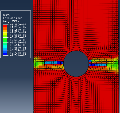
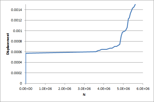
The plot of SDV2 depicts the cycles to failure for each element. You can also use nodal displacements and the cycles to failure for unfailed regions of the model to create a plot of cycles to global structural failure as seen below.