Graph Area

Below is an image of the Graph Area. This graph will only appear after a stress classification line (SCL) has been defined using the Linearization Controls.

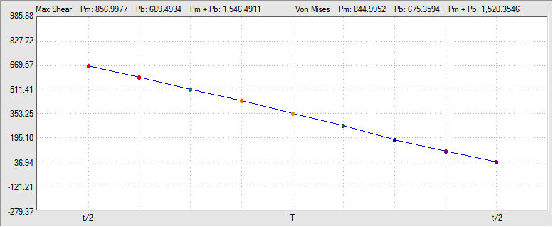
The SCL is divided into segments. The results are calculated from the stress tensor values and output at each point. The number of points defined along the line is equal to the number of elements intersected by the SCL plus one. SCL Point #1 is Node 1 and the last SCL Point is Node 2. Node 1 is at -t/2 in the graph and Node 2 is at t/2. The origin of the local N, T, H coordinate system is at the center of the SCL at point T. If the SCL goes through an area of space where there is no model, then no data points exist along that portion of the SCL. If you hover the mouse over a point on the graph, the following pop-up information box appears. The toolbar buttons at the left of the graph area allow you to specify which local stress tensor to display. For information on the T, N, and H axes, see Linearization Controls. The units for the graph depend on the unit system of your model (force/length²).

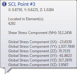
This pop-up information box tells you the global coordinates of the SCL and what elements it is located in. It also includes the local stress tensor that is currently being displayed on the graph and the six global stress tensors.

Above the graph, six additional results are listed:

• Max Shear: (Combined membrane and bending stresses based on the maximum shear stress method):
  • P_m: This is the general primary membrane stress intensity.
  • P_b: This is the primary bending stress intensity.
  • P_m + P_b: This is the sum of the general primary membrane stress intensity and the primary bending stress intensity.
• Von Mises: (Combined membrane and bending stresses based on the Von Mises stress method):
  • P_m: This is the general primary membrane stress intensity.
  • P_b: This is the primary bending stress intensity.
  • P_m + P_b: This is the sum of the general primary membrane stress intensity and the primary bending stress intensity.

P_m and P_b are calculated based upon the variation of the primary stress along the SCL. For more information, see the page How to Calculate Pm and Pb.

Note: The graph is most meaningful, and corresponds well with the listed P_m, P_b, and P_m + P_b values, if...

• the local N, or H axis is appropriately defined, and
• the appropriate tensor (NN, TT, HH, NT, TH, or NH) is selected for graphing.

  Ideally, the graphed stress tensor should correspond with the direction of the primary membrane and bending stresses.