Graph Area

Below is an image of the Graph Area. This graph appears only after a stress classification line (SCL) has been defined using the Define Points and Perpendicular Direction inputs.

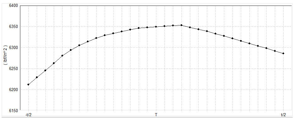
The SCL is divided into segments. The results are calculated from the stress tensor values and output at each point. The default number of points defined along the line is determined automatically by the program. You can also override the default behavior by specifying the desired number of SCL divisions (see Define Points and Perpendicular Direction). SCL Point #1 is the First Point, and it is at located at -t/2 in the graph. The Last Point is located at t/2. The origin of the local N, T, H coordinate system is at the center of the SCL at point T.

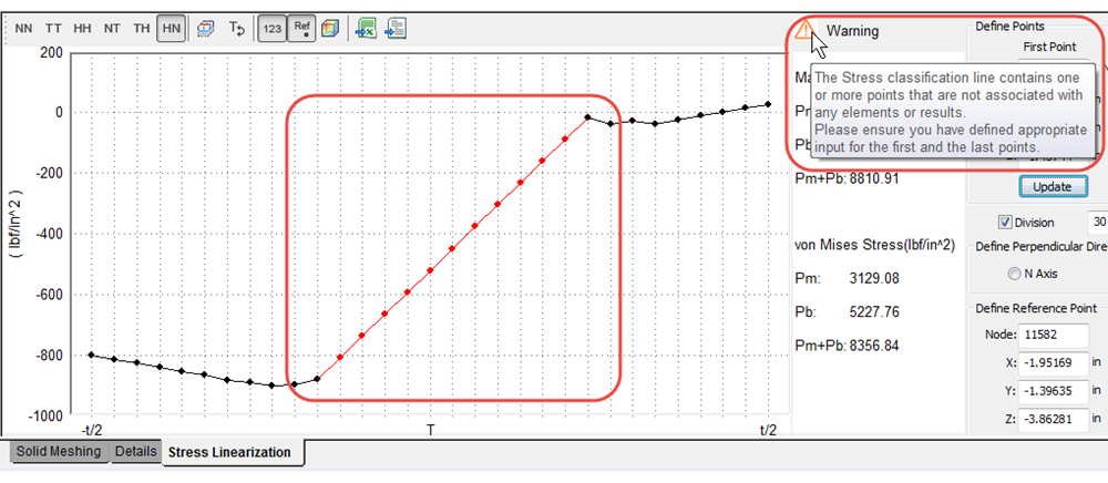
If the SCL goes through an area of space where there are no elements, the data points along that portion of the SCL are interpolated from the nearest valid data points. In such cases, the curve and data points are red for the portion of the graph that is outside of the model elements. In addition, a Warning symbol appears at the top right corner of the graph area. Point to this notification with the cursor to see a pop-up message describing the problem. The following image shows an example of a graph with a portion of the curve in red and the associated warning message:

The leftmost set of toolbar buttons above the graph area allow you to specify which local stress tensor to display. The units for the graph depend on the currently active unit system of your model (force/length²).

If you hover the cursor over a point on the graph, the following pop-up information box appears:

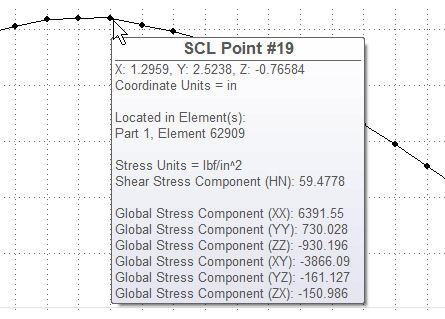
This box tells you the global coordinates of the SCL point and the part and element numbers at the point location. It also includes the local stress tensor that is currently being graphed and the six global stress tensors from which the stress linearization results are derived.

Note: The graph is most meaningful, and corresponds well with the listed Pm, Pb, and Pm + Pb values, if the following conditions are satisfied:

• The local N, or H axis is appropriately defined.
• The appropriate tensor (NN, TT, HH, NT, TH, or HN) is selected for graphing.

  (Ideally, the graphed stress tensor should correspond as closely as possible to the direction of the primary membrane and bending stresses.)