The following are all of the toolbar buttons available in the Stress Linearization tab of the Output Bar, and the functions that they perform. Many of these buttons function as toggles (click once to activate; click again to deactivate). The visual state of each button changes to indicate when the option is active.
- Local Stress Tensors –
 ,
,
 ,
,
 ,
,
 ,
,
 , and
, and

- Click one of these six buttons to choose which local stress tensor result to plot in the graph area.
- The first letter of the tensor refers to the vector normal to the face of the element. This vector corresponds to the face of an ideal element transformed to the local coordinate system; it does not necessarily correspond to the actual element faces.
- The second letter is the direction of the stress.
- For example, NN is the normal stress in the local N direction and TH is the shear stress along the HN plane in the H direction.
- The SCL must be defined before a graph is displayed; and the N, H, and T axes should be properly oriented. For information on how these direction are defined, refer to the Define Points and Perpendicular Direction page.
 – Show Intersected Elements Only
- This option affects the appearance of the model within the display canvas of the Results environment. It does not affect the contents of the Stress Linearization tab within the Output Bar.
- Activate this option to hide all of the elements of the model that are not intersected by the SCL. Only the intersected elements remain visible. (See Figure 3.)
Note: When the Show Intersected Elements Only option is first activated, the Show Internal Mesh option is also activated in the Results environment (Results Options
 View Show Internal Mesh).
 – Invert T Axis
- Activate this option to reverse the positive direction of the T axis. When not activated, the T axis points from the First Point of the SCL to the Last Point of the SCL. When activated, the T axis points from the Last Point of the SCL to the First Point of the SCL.
 – Show SCL Numbers
- This option affects the appearance of the model within the display canvas of the Results environment. It does not affect the contents of the Stress Linearization tab within the Output Bar.
- In the model display area, a yellow dot appears along the SCL at each calculation point. Activate this option to display the identification number of each of these calculation points. The points are numbered sequentially from the First Point to the Last Point, beginning with 1. (See Figure 3.)
 – Show Reference Point
- This option affects the appearance of the model within the display canvas of the Results environment. It does not affect the contents of the Stress Linearization tab within the Output Bar.
- Activate this option to show the reference point within the model display area. The reference point is displayed as a small dark-pink sphere. (See Figure 3.)
 – Display Elements Transparently
- This option affects the appearance of the model within the display canvas of the Results environment. It does not affect the contents of the Stress Linearization tab within the Output Bar.
- Pressing this button will cause the model to be shaded with the mesh lines. The color of the shading will follow the contour of the selected stress tensor. (See Figure 3.)
 – Save Values to CSV File
- Click this button to save a table of your stress linearization results as a *.csv file (comma-separated values). This file format can be opened in Microsoft Excel (See Figure 1) or in any plain text editor. The exported table contains the following information:
- Model path and filename
- Design Scenario identification
- Load Case identification
- Coordinate Units
- Stress Units
- Coordinates of the First, Last, and Reference Points (defining the SCL)
- Pm, Pb, and Pm+Pb based on the Von Mises stress
- Pm, Pb, and Pm+Pb based on the maximum shear stress
- A stress tensor table with the following columns (and one row of data per calculation point along the SCL):
- Point ID
- X, Y, and Z coordinates
- All six stress tensors based on the local coordinate system (NN, TT, HH, NT, TH, and HN)
- All six stress tensors based on the global coordinate system (XX, YY, ZZ, XY, YZ, and ZX)
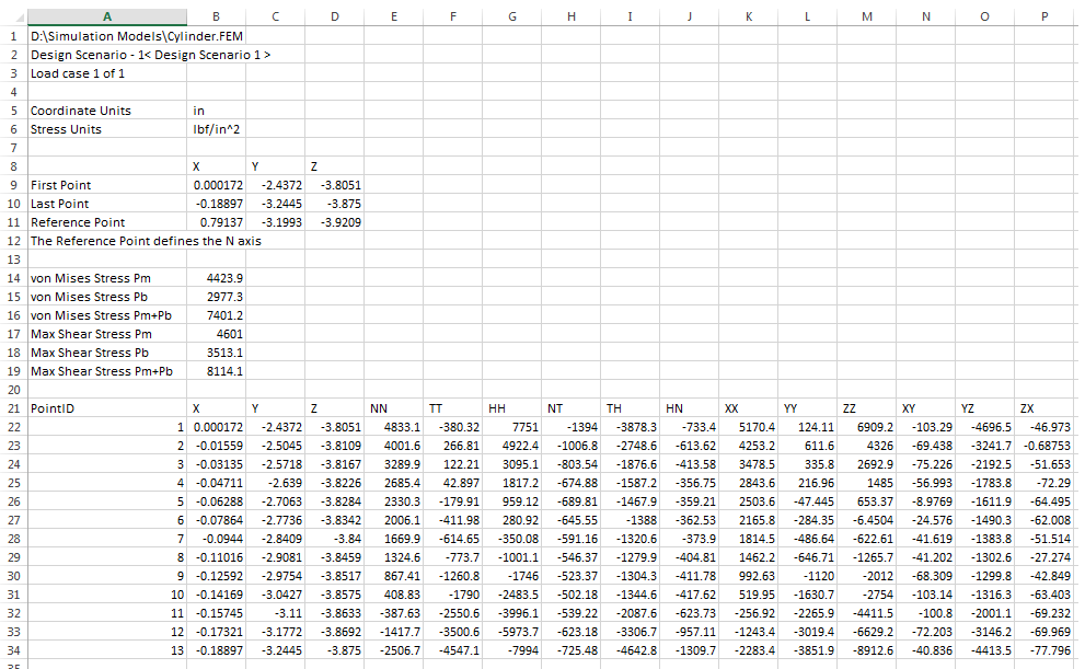
- Figure 1: Sample CSV File (as viewed in Microsoft Excel)
 – Save Results to Report
- Click this button to save the stress linearization results to an output file (*.scl) and to automatically add these results to your HTML report for the analysis (See Figure 2). The report includes the following data:
- Stress Linearization Input Data
- X, Y, and Z coordinates of the first, last, and reference point on which the SCL is based
- Identification of the axis defined by the reference point (N or H axis)
- Local stress tensor graph (based on the currently selected tensor component)
- Pm, Pb, and Pm+Pb based on the Von Mises stress
- Pm, Pb, and Pm+Pb based on the maximum shear stress
- Stress Linearization Input Data
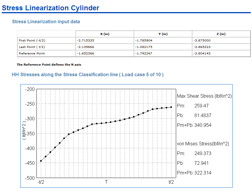
- Figure 2: Sample Stress Linearization Report (part of the analysis HTML report)
Model Appearance for a Stress Linearization Example
The following figure is an example of the model appearance for a stress linearization computation, with active options as listed below the figure:
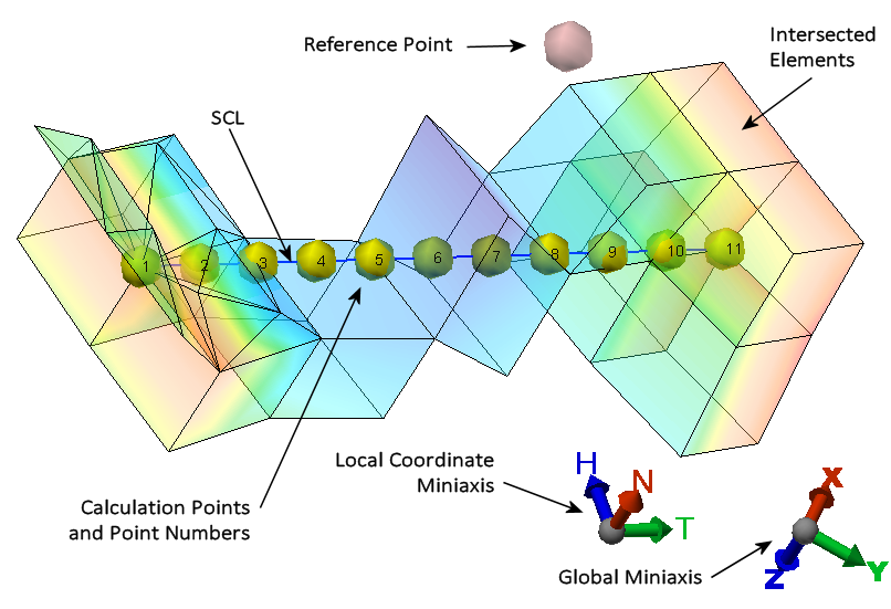
Figure 3: Sample Model Appearance with the Following Options Enabled:
- – Show Only Intersected Elements
- – Show SCL Numbers
- – Show Reference Point
- – Display Elements Transparently