In order to consider the pump for simulation purposes it has to be presented in a form that satisfies equation the work energy equation.
The head versus flow rate curve needs to be represented mathematically on the computational domain in the same form as the frictional and minor losses. In order to do this the pump curve needs to be expressed in the form of a polynomial equation. However, the pump provides pressure to the network so it is modeled as a negative flow resistance, and the sign is reversed:

where
 or h represent pressure drop, the various Ks are variables that are dependent on the empirically determined pressure-drop flow-rate relationship used, and Q is the volumetric flow rate.
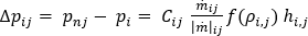
Solving the work energy principle equation on the coolant flow computational domain, the pressure drop relationship for any of the branch elements of node [ i ] can be expressed by:
where
 is the pressure drop flow rate relationship derived from the work energy principle,
 is the connectivity operator, (+) or (-),
 is the mass flow rate, and
 is a function of the density of the fluid in the network. For incompressible fluids, such as water, this is a constant.
When expressing the polynomial equation in its final discretized form, and subsituting it into the work energy equation for any of the branch elements of node [i], the pressure loss associated with a pump is given by:
