The following examples show how to interpret profiles based on graph colors and categories, and how each performance optimization in Maya can impact a scene's performance. The following examples are all generated from the same simple FK character playback in Maya 2019.
DG Evaluation
- Pink and purple Dirty Propagation events in the Dirty Propagation category.
- Dark green Pull Evaluation events in the Evaluation category.
- Blue VP2 Pull Translation and light blue VP2 Rendering in the VP2 Evaluation category.
- Yellow events in the VP2 Evaluation category show the time VP2 spent waiting for data from Dependency Graph nodes.
In this example, a significant fraction of each frame is spent on Dirty Propagation, a problem you can address with the Evaluation Manager.
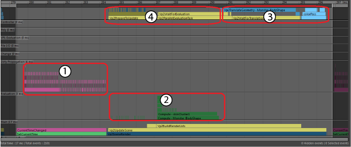
EM Parallel Evaluation
- Peach, tan, and brown EM Parallel Evaluation events of the FK rig colored. The high stack of events represents some evaluation occurring in parallel.
- Tan and brown EM Parallel Evaluation events occur when Maya evaluates the skin cluster to compute the deformed mesh. These events occur serially because the Dependency Graph has no parallelism.
- Dark blue and blue VP2 Direct Update events translate data into a VP2 render-able format.
- Yellow in the Main category and light blue in the VP2 Evaluation category are VP2 Rendering events.
In this example, much less time is spent on Vp2SceneRender (4). This occurs because time spent reading data from dependency nodes has moved from rendering to EM Parallel Evaluation (1 and 2). DG evaluation uses a data pull model, while EM Evaluation uses a data push model. Additionally, some geometry translation (3), is also moved from rendering to evaluation. We call geometry translation during evaluation "VP2 Direct Update".
A significant portion of each frame is spent deforming and translating the geometry data, a problem you can address with GPU Override. See GPU Override in Increase performance with the Evaluation Manager.
EM Parallel Evaluation with GPU Override

- Light and dark yellow GPU Override events have replaced the long serial central part of the EM Parallel Evaluation profile (2 & 3 from EM Parallel Evaluation). These GPU Override events represent the time the CPU takes to marshal data and launch the GPU computation.
- Peach, tan, and brown EM Parallel Evaluation events here have roughly the same duration as EM Parallel Evaluation, even though the relative size of the rig evaluation events with GPU Override is larger. This size difference is because the scale of this profile is different from the scale of the previous profile, 5 milliseconds versus 12 milliseconds.
- Light blue VP2 Render events have experienced a similar relative stretching (2).
EM Evaluation Cached Playback
- Yellow Restore Cache events record the time it takes to update each FK rig node which has cached data. There are also brown VP2 Direct Update events that track update of the VP2 representation of the data.
- Yellow Restore Cache event for the deformed mesh. This represents the time taken to restore the data into the Maya node, and to translate the data into VP2 for drawing using VP2 Direct Update.
EM VP2 Hardware Cached Playback
- Dark blue VP2 Hardware Cache Restore events replace the long serial Cache Restore event (#2 from EM Evaluation Cached Playback, the section above). Restoring the VP2 Hardware Cache is much faster because the data is already in render-able format and stored on the GPU.
- Gray Cache Skipped event shows that data in the dependency node is not updated.
Evaluation-Bound Performance
A scene is considered Evaluation-bound when the main bottleneck in your scene is evaluation. There are several problems that may lead to evaluation-bound performance.
- Lock Contention
- Lock Contention occurs when many threads try to access a shared resource, due to lock management overhead. You can identify this occurrence when evaluation takes roughly the same duration no matter which evaluation mode you use. Lock Contention occurs when threads cannot proceed until other threads are finished using the shared resource.
-
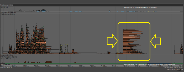
- The above image shows many identical tasks starting at nearly the same time on different threads, each finishing at different times. This type of profile suggests there might be a shared resource that many threads need to access simultaneously.
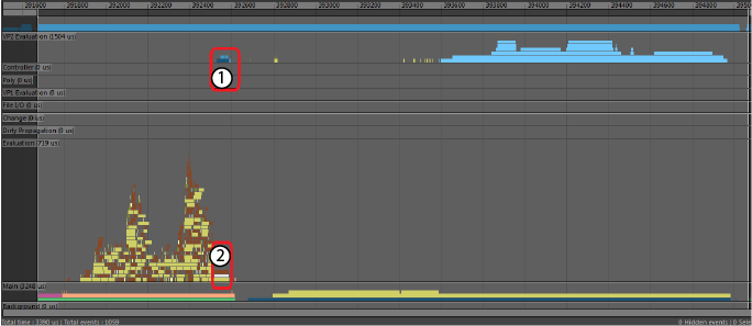
- Below is another image that shows a similar problem:
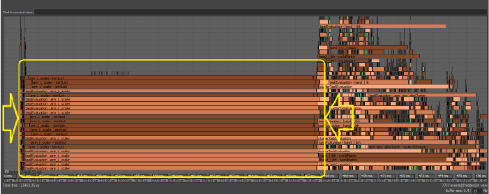
- In this case, since several threads were executing Python code, they had to wait for the Global Interpreter Lock (GIL) to become available. Bottlenecks and performance losses caused by contention issues may be more noticeable when there is a high concurrency level, such as when your computer has many cores.
If you encounter contention issues, try to repair the affected code. In the above example, changing the node scheduling converted the above profile example to the following one, which shows a performance gain. For this reason, Python plug-ins are scheduled as Globally Serial by default, which means they are scheduled one after the other and do not block multiple threads waiting for the GIL.
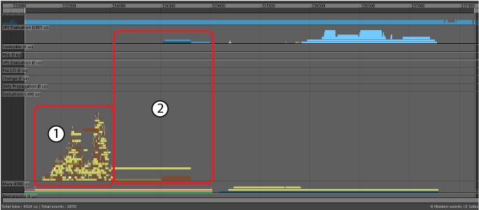
- Clusters
- If the Evaluation Graph contains node-level circular dependencies, those nodes are grouped into clusters that represent single units of work to be scheduled serially.
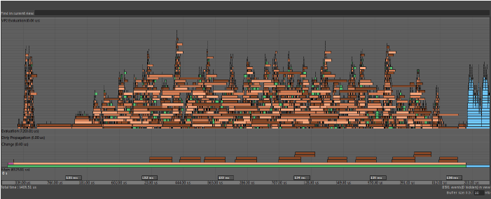
- Although multiple clusters can evaluate at the same time, large clusters limit the amount of work that can be performed simultaneously. Clusters can be identified in the Profiler as bars with the opaqueTaskEvaluation label, shown below:
-

- If your scene contains clusters, analyze the rig structure to locate any circularities. Ideally remove coupling between parts of the rig, so rig sections (for example, head, body, and so on,) can evaluate independently.
Tip: Disable costly nodes using the per-node 'frozen' attribute in the Evaluation Toolkit when troubleshooting scene performance issues. This lets you temporarily remove specific nodes from the Evaluation Graph, and gives you a simple way to know if you have located the correct bottleneck in your scene.
Render-Bound Performance
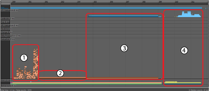
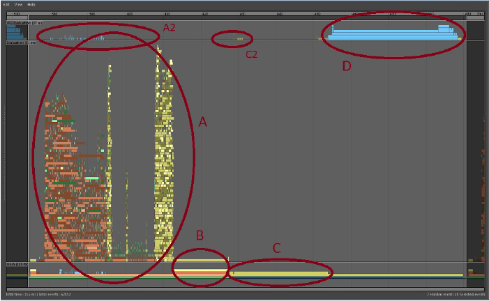
A scene is render-bound when the main bottleneck in your scene is rendering. The following Profiler example is expanded to a single frame taken from a large scene with many animated meshes. Because of the number of objects, different materials, and the amount of geometry, this scene is very costly to render.
-
- Evaluation
- GPUOverridePostEval
- Vp2BuildRenderLists
- Vp2Draw3dBeautyPass
In this scene, many meshes are being evaluated with GPU Override so some Profiler blocks appear differently from what they would otherwise.
- Evaluation
- Area A shows the time spent computing the state of the Maya scene, which in this case, is moderately well-parallelized. The blocks in shades of orange and green represent the software evaluation of DG nodes. The yellow blocks are the tasks that initiate mesh evaluation via GPU Override. Mesh evaluation on the GPU starts with these yellow blocks and continues at the same time as the other work on the CPU.
- An example of a parallel bottleneck in the scene evaluation appears in the gap in the center of the evaluation section. The large group of GPU Override blocks on the right depend on a single portion of the scene and must wait until it is complete.
- Area A2 (above area A), are blue task blocks that show the work that VP2 does in parallel with the scene evaluation. In this scene, most of the mesh work is handled by GPU Override so it is mostly empty. When evaluating software meshes, this section shows the preparation of geometry buffers for rendering.
- GPUOverridePostEval
- GPU Override finalizes some of its work in Area B. The amount of time spent in this block varies with different GPU and driver combinations. At some point, there is a wait for the GPU to complete its evaluation if it is heavily loaded. This time may appear here, or it may show as additional time spent in the Vp2BuildRenderLists section.
- Vp2BuildRenderLists
- Area C. Once the scene is evaluated, VP2 builds the list of objects to render. Time in this section is proportional to the number of objects in the scene.
- Vp2PrepareToUpdate
- Area C2 is very small in this profile. VP2 maintains an internal copy of the world and uses it to determine what to draw in the Viewport. When it is time to render the scene, we must ensure that the objects in the VP2 database have been modified to reflect changes in the Maya scene. These may be, for example, objects that have become visible or hidden, had their position or their topology change, and so on. This is done by VP2 Vp2PrepareToUpdate.
- Vp2PrepareToUpdate is slow whenever there is shape topology, material, or object visibility changes. In this example, Vp2PrepareToUpdate is almost invisible since the scene objects require little extra processing.
- Vp2ParallelEvaluationTask is another Profiler block that can appear in this area. If time is spent here, then object evaluation has been deferred from the main evaluation section of the Evaluation Manager (area A) to be evaluated later. Evaluation in this section uses traditional DG evaluation.
- Common cases that slow Vp2BuildRenderLists or Vp2PrepareToUpdate during Parallel Evaluation are:
- Large numbers of rendered objects (as seen in this example)
- Mesh topology changes
- Object types, such as image planes, that require legacy evaluation before rendering
- 3rd party plug-ins that trigger API callbacks
- Vp2Draw3dBeautyPass
- Area D. Once all data has been prepared, the scene is rendered. This is where the OpenGL or DirectX rendering occurs. This area is broken into subsections depending on Viewport effects such as depth peeling, transparency mode, and screen space anti-aliasing.
- Vp2Draw3dBeautyPass can be slow if your scene:
- Has Many Objects to Render (as in this example).
- Uses Transparency Large numbers of transparent objects can be costly since the default transparency algorithm makes scene consolidation less effective. For very large numbers of transparent objects, setting Transparency Algorithm (in the VP2 settings) to Depth Peeling instead of Object Sorting may be faster. You can also switch to untextured mode to bypass this cost.
- Uses Many Materials In VP2, objects are sorted by material before rendering, so having many distinct materials makes this time-consuming.
- Uses Viewport Effects Many effects such as SSAO (Screen Space Ambient Occlusion), Depth of Field, Motion Blur, Shadow Maps, or Depth Peeling require additional processing.
- Other Considerations
- Although the key phases described above apply to all scenes, your scene may have different performance characteristics.
- For static scenes with limited animation, or for non-deforming animated objects, use consolidation to improve performance. Consolidation groups objects that share the same material and reduces time spent in both Vp2BuildRenderLists and Vp2Draw3dBeatyPass, since there are fewer objects to render.
Saving and Restoring Profiles
Profile data can be saved at any time for later analysis using or in the Profiler window. Everything is saved as plain string data so that you can load profile data from any scene using without loading the scene that was profiled.