External Incompressible Flow
External flows are characterized by a solid body immersed in fluid that is moving relative to the body. Nearly all engineering aerodynamic problems are external flows. Examples include noise generated by a car mirror at highway speeds, the drag on a motorcycle fairing, and the lift on a missile. Additionally, wind tunnel models are usually considered external flows.
These problems generally require the greatest number of nodes of any CFD calculation since the velocity and pressure boundary conditions applied at the exterior of the flow domain must not affect flow features around the immersed body.
Calculation Domain Size
Generally, the exterior or “far-field” boundary must be at least 5 to 10 chords upstream and 10 to 20 chords downstream of the body. Higher Reynolds number flows will require far-field distances in the upper portion of this range.
Meshing Strategy
It is important to transition the element sizes in the mesh quite substantially to conserve nodes. It is common for elements on the body surface to be several thousand times smaller than elements at the far-field. Lift and drag forces calculated by Autodesk® CFD will be dependent upon the mesh size near the body.
Transitioning must be smooth for solution stability and accuracy, and care must be taken to avoid creating tetrahedral elements with very high aspect ratios. Sometimes embedding fluid volumes using mesh refinement regions around the object of interest is very useful for concentrating many elements around it. This approach helps transition the mesh from very small elements around the object to larger elements further away from the object.
Boundary Condition Placement
For incompressible and subsonic compressible flow problems with subsonic inlets, velocity and pressure boundary conditions are applied on the far-field boundary as shown in the following figure. To aid convergence, it is useful to specify the velocity boundary condition around a greater portion of the flow domain than for pressure, as shown in the following figure:
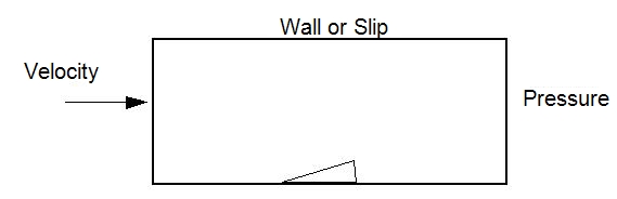
Apply slip conditions to any surfaces that are not openings unless the boundary layer or ground effects are of interest against the wall.
Angle of Attack
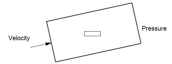
If the object has an angle of attack relative to the flow, it is better to re-orient the calculation domain instead of the object. The domain orientation should be that the free-stream velocity and the domain sides are parallel:
Simulation Recommendations
We recommend these techniques to improve accuracy of the drag calculation:
Mesh
The region around the object must be meshed with a very fine mesh. More streamlined bodies require the mesh near the stagnation point of the body to be highly refined to capture the rapidly changing coefficient of pressure.
Wall Layers
Specify at least 10 layers on the Wall Layers dialog:
Click Setup > Setup tasks > Mesh Sizing.
From the context menu, click Wall Layers.
Drag the Number of layers slider to 10.
Drag the Layer gradation slider from Auto to 1.5. (This positions the first element layer very close to the wall, helping to satisfy the Y+ requirements of the SST model.)
Turbulence Model
Invoke the SST k-omega turbulence model:
- Open the Solve dialog, and click Turbulence on the Physics tab.
- From the Turb. model menu, select SST k-omega.
Advection Scheme
Invoke the ADV5 advection scheme.
- Open the Solve dialog, and click Solution control on the Control tab.
- On the Solution Controls dialog, click Advection.
- Select ADV 5 from the list.
Mesh Adaptation
Enable Mesh Adaptation. This option progressively refines the mesh over the course of several iterations of the simulation. The result is a mesh-independent solution. Note that this option can be computationally intensive, and can take longer than a single execution of the mesh.
- Open the Solve dialog, and click the Adaptation tab.
- Check Enable Adaptation.
- Expand the Additional Adaptation list, and enable Y+ Adaptation. Reduce the Max Y+ to 10 to ensure that the SST turbulence model has an acceptable working range for all wall surfaces.
- Enable the options for Flow Angularity, Free Shear Layers, and External Flow.
Convergence
Note that convergence will often be slow, and the monitor will show relatively flat lines well before the flow field is fully developed around the body. Subtle differences in the pressure distribution may not be visible by only reviewing the convergence monitor.
To adjust the Automatic Convergence Assessment to Tight, on the Control tab of the Solve dialog, click Solution Control. Click the Advanced button in the Intelligent Solution Control group. Move the slider to Tight.
Altitude Effects
To simulate the effect of altitude, we recommend that you consult tables of atmospheric data to identify the static pressure and temperature based on a geometric and/or geopotential altitude. From the pressure and temperature, the density of the air can be computed and specified as a constant property.
If properties are held constant (hence you are not solving for compressible or thermal effects) the density is the only parameter that needs to be modified on the Material Editor. Keep in mind that the actual effect that is simulated at different altitudes is that of the Reynolds number.
Related Topics: