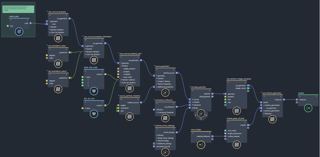
The following illustration shows the top level of a sample particle graph. All Bifrost graphs have similar elements.

Data flow

Bifrost is a pure data flow graph. Data flows "downstream" from left to right along connections between ports on nodes.

The inputs may be coming from the host scene through input nodes, such as scene geometry or numeric parameters. Alternatively, they can be created inside the graph itself, for example, with value nodes or simple geometry-creation nodes like create_mesh_sphere.

The results of the graph computation are sent to the scene through a connection to an output or terminal node. Most graphs output Bifrost geometric objects, which create bifrostGraph objects in the scene. These can be displayed in the viewport, as well as rendered with compatible renderers such as Arnold.

By default, graphs have one input node and one output node. However you can create additional input and output nodes in the same way as any other node.

Alternatively, Bifrost graphs can output geometry to standard formats like Alembic and VDB for use with other renderers. See Input and output data from files.

Nodes

Nodes perform operations on their inputs, and output the results. The input ports are on the left, and the output ports are on the right.

There are nodes for basic functions like add and multiply. There are also high-level nodes like simulate_particles that perform many operations to create an effect, as well as medium-level nodes that serve as useful utility functions.

The high-level and medium-level nodes are usually compounds. Compounds are nodes that contains subgraphs of other nodes and possibly even other compounds. You can double-click on a compound to enter it and view its contents. You can also create your own compounds to organize your graphs, as well as to publish them for reuse — see Create and edit compounds.

Published compounds that you add to a graph are referenced by default. This means that they refer to a node definition on disk. You cannot modify the internal subgraph of a referenced compound until you import it locally into a graph — see Import a referenced compound.

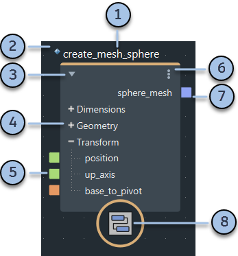
1. Node name or value. The default name is based on the node's type, but you can double-click on the name to type a new one — if values are currently displayed instead of names, you may need to first choose Display > Show Node Names while the node is selected. To display the type of nodes above their names, press T or choose Display > Show Node Types.
2. Diamond icon. This indicates that the node is a referenced compound. Referenced compounds contain subgraphs that have been published for reuse. You cannot modify their internal graphs unless make them editable — see Import a referenced compound.
3. Click the triangle to collapse or expand the node. Alternatively, you can use the 1, 2, and 3 hotkeys, or commands on the Display menu. When a node is collapsed, its individual ports are not displayed.
4. Port groups. Click + or – to expand and collapse.
5. Input ports. Connect the outputs of other nodes, or enter values in the Parameter Editor. Right-click for other options.
6. Node menu. You can also right-click on the main body of nodes.
7. Output port. Connect to the inputs of other nodes. Right-click for other options.
8. Node icon. Some nodes may have special icons related to their function. The icon shown above is the default for compounds. In most cases, the icon simply helps with readability and recognition in the graph, but be careful when using nodes with the experimental icon (an orange overlay of a laboratory flask) — see About experimental nodes.