Modal analysis determines eigenvalues and derivative values (eigenpulsations, eigenfrequencies or eigenperiods), precision, eigenvectors, participation coefficients and participation masses for the problem of structure eigenvibrations.
Three structure dynamic analysis modes (modal, seismic and seismic (pseudo)) are available.
Eigenvalues and eigenmodes are obtained from the following formula.
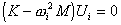 (1)
(1)
where:
K - stiffness matrix of the structure,
M - mass matrix of the structure,
ωi - natural pulsation (natural circular frequency) of mode "i",
Ui - eigenmode vector of mode "i".
The number of eigenmodes to be considered can be specified as follows.
- The upper limit of the pulsation, frequency or period.
- The lower limit of the sum of participation masses (percentages) or as a real number of required modes.
If the mode number is not specified, the default value set in Preferences is used in the analysis.
Control parameters for the eigenproblem algorithm are as follows.
- Precision of calculations (error quantity).
- Maximum number of iterations.
The following mass matrix types are available.
- Consistent (consistent matrix - always with regard to rotational degrees of freedom),
- Lumped with rotations (diagonal matrix - with regard to rotational degrees of freedom),
- Lumped without rotations (diagonal matrix without rotational degrees of freedom).
Lumped mass matrices Mlum are created in accordance with the rule:
Mlum(i,j) = 0.0 ; for i≠j
Mlum(i,j) = Stot/Sdiag * M(i,j) ; for i=j (2)
where:
Stot - Sum of all elements of consistent mass matrix M,
Sdiag - Sum of diagonal elements of consistent mass matrix M.
Thus, the element mass is preserved and the element mass matrix is positive definite.
Eigenvectors in the result modules are normalized so that the maximum term of each vector equals 1.0.
Internal eigenvectors used during calculations are normalized so that
 (3)
(3)
The precision value displayed in the eigenvalue dialog is regarded as an achieved accuracy of convergence. This value is an acceptable error quantity for how precisely the eigenvalue λi and the eigenvector Ui achieved during iteration for the i-th mode satisfy the eigenproblem equation:
K * Ui = λi * M * Ui (4)
Participation coefficients are defined as:

where:
D - Unit vector defined as follows:
D(j) = 1.0 if j is equal to the i-th degree of freedom
D(j) = 0.0 if j ¹ i,
Vi - Eigenvector of mode i normalized in the way that 
Participation masses are dynamic, participating in the motion of the structure for each mode and each degree of freedom. They are regarded as the current masses for the current mode and as the relative masses which are the sum of the current masses from the first mode to the current one. Values are presented as a percentage of the total dynamic masses.
Current participation masses are defined as follows:

Presently, the Lanczos' Algorithm, which constitutes a powerful approach to solve large scale eigenvalue problems (1), is the default method of finding the eigenproblem solution. It finds the required n eigenvalues and eigenvectors with any accuracy.
For most cases the Lanczos' Method is preferred as the most adequate. However, the following restrictions apply.
- Tridiagonal matrix T should not be of a consistent type.
- Mass matrix M should be treated as Lumped with Rotations or Consistent. When Lumped without Rotations is selected, the mass matrix is automatically aggregated as Lumped with Rotations.
When in a program a Lanczos' method is selected, the program changes a calculation method to a subspace iteration method. To use the Lanczos' method in calculations, separated structures should be connected in such a way that a structure model is not changed (for example, a bar among the supports should be added).
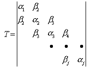
The following reduction of the tridiagonal matrix T applies in the Lanczos' Method.
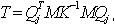
where
Qj = {q1, q2, ... , qj} - rectangular matrix Neq x j, Neq - number of equations, j - number of Lanczos' steps, qj - j-th Lanczos' vector.
The formula
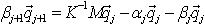
is used to generate the next Lanczos' vector qj+1 and sets the current line of the matrix T.
Thus, the reduced eigenproblem is:
 , k=1,2,…,j
 , where ωk j is the j-th approximation to ωk, k=1,2,…,n, and n is the required number of eigenvalues and eigenvectors. An algorithm will carry on the calculations (increasing the j - number of Lanczos' steps) till the required accuracy for all n eigenvalues is achieved.
The orthogonalization procedure supports the required level of orthogonality between the Lanczos' vectors, ensuring the safeness and the numerical stability of calculations.
Eigenvectors are to be obtained from the following formulas:
U = Qs.
Basis Reduction Method
The Basis Reduction Method obtains approximate values of the first few eigenvalues, provided some data about them are already gathered. This method requires assigning master degrees of freedom (MDOF) to get the reduced system. Governing the creation of the reduced model is then possible and undesirable degrees of freedom can be excluded from the reduced model which will result in a significantly smaller system. It is especially useful for those with some experience in structure dynamic analysis and when the dynamic structure behavior is known.
The following rules apply to this method.
- MDOF have to be specified (master nodes and directions). It is assumed that only displacements (not rotations) can be assigned as master degrees of freedom.
- Any mass matrix type can be used in the algorithm. However, the Lumped without Rotations matrix type ensures the shortest calculation period.
- Sturm Check indicates the number of skipped frequencies. These values and eigenvectors will not be found. The only way to find the verification convergence is to increase the number of MDOF in order to resolve the problem and compare eigenvalues.
The method includes transformation of the large eigenproblem for the FEM model.
K U - ω2 M U = 0 to the eigenproblem for a reduced model:
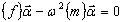
where {f} - influence matrix, {m} - generalized matrix for the reduced model.
The basis for such transformations are the solutions obtained for appropriate unit states:
unit nodal forces are applied consequently for each node of master type in the selected direction of master type. The large scale static problem has been solved for n right sides:
K Xi * = Ti , i = 1, 2, …, n
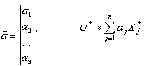
where Ti - load vector corresponding to the i-th unit force. Nodes and directions of mastertype are to be defined, all other operations will execute automatically. Then, the reduced eigenproblem is solved with the Jacobi's Method. As a result, the approximate values of frequencies wi and eigenvectors Ui * , i=1,2,…,n are obtained.
See also:
Modal Analysis - Precision of Calculations in Structural Modal Analysis