Learning Objectives

• Change the number of solving iterations.
• Specify the balancing and terrain smoothing objective weights.
• Initiate an optimisation.
• Review and analyse the solution through the Convergence Plot.
• Conclude more constraints are necessary.

Open Grading Optimization

In the previous exercise, Creating Grading Limits, you specified a grading object and are now ready to open the object and its surface in Grading Optimization.

In Civil 3D, Click Analyse tab > Grading Optimization panel > Optimise.

If multiple surfaces are in the drawing, you will be prompted to select the surface that you would like to use as the existing ground.

Grading Optimization opens. The surface and the Grading Limit object you previously created are displayed in the Visualisation Display.

Specify Objectives and Solver Settings

You will now configure the objectives that were explored in the exercise Optimisation Constraints.

On the bottom right of Grading Optimization, on the Optimisation Toolbar, click Optimisation Options to open the Optimisation Options dialog.

Specify Global Constraints

The Global Constraints settings specify global slope constraints for both the maximum allowed slope and the minimum required drain slope. These values are used in two specific situations:

1. When a grading limit is not applied.
2. When a zone lacks custom slope settings and has the Use global settings property enabled.

To make certain that a required minimum drain slope is not active on new zones added in the future, change that global setting to zero.

Specify Optimisation Settings

The Optimisation settings define the number of solver iterations will be calculated.

Limit the number of iterations to 25,000. This will terminate the solving process much earlier.

Define Objective Weights

You will now specify objectives as discussed in the exercise Optimisation Objectives. There are two main objectives for the mass grading:

• Terrain Smoothing
• Balancing cut and fill

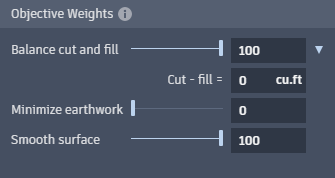
In the optimisation settings, you can specify the relative weights for each, on a scale from 0 to 100. To select a target balance volume, click the arrow to the right of Balance cut and fill.

For the purpose of this exercise, leave it at 0 cu.ft.

Give each objective equal weight and turn both to 100. Leave the earthwork minimisation at 0, as you do not want to stay as close as possible to the existing ground.

When you have completed the optimisation settings, close Optimisation Options dialog.

Run an Optimisation

Now, you will observe an optimisation and prepare to analyse your grading settings.

On the bottom right of Grading Optimization, click Optimise to begin the optimisation.

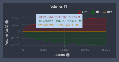
Notice that the solver starts changing the terrain contours in the Visualisation display. Click on either the Violation tab or Cut-fill tab of the Optimisation Panel to open the Convergence Plots dialog.

You can now observe how the optimisation solver progresses as previously explained in Optimisation Constraints. The following picture shows the feasibility plot after 25,000 iterations.

As the proximity value becomes smaller, notice that the solver is trending closer towards a feasible solution. Allowing this optimisation to run longer, you can see the proximity value keeps moving towards zero. This indicates there is a unique feasible solution, which is also the best solution referencing the current objectives. The balancing plot shows a perfect balance.

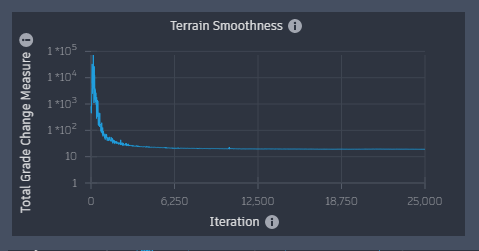
The cut and fill volumes are still growing as expected. Minimisation of the earthwork is not required, so the solver is creating more volumes to better smooth the surface and create contours that are more easily graded with machinery. The plot for terrain smoothing are also visible.

Analyse the Results

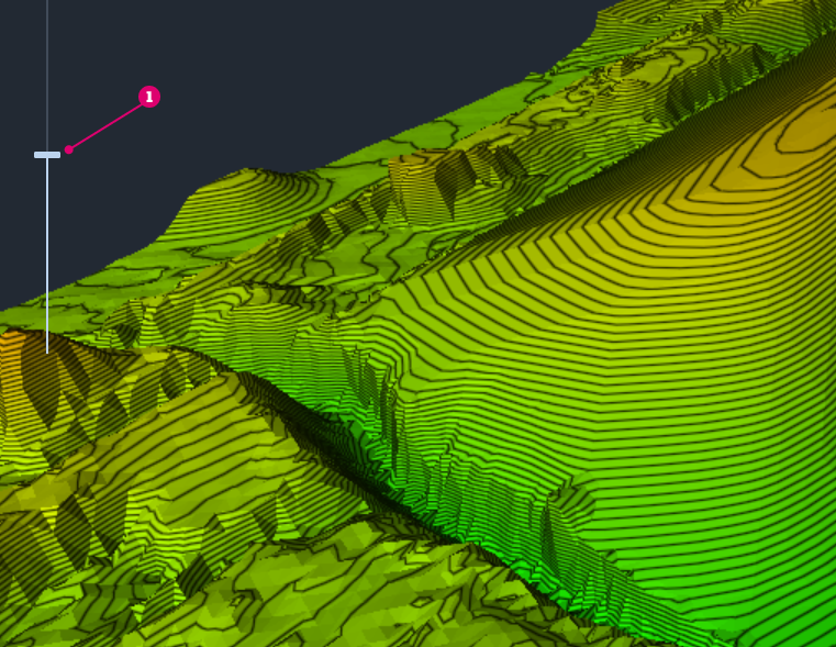
When looking at the final surface in the Grading Optimization Visualisation Display, notice that the net volume is at -62,473 cubic feet, which corresponds to about -2,314 cubic yards.

Assuming a dump truck carries on average 15 cubic yards, 155 trucks of fill are required.

The contours on the surface show a hill on the left side that slopes the terrain down to the specified 33%. This is better visualised by exaggerating the elevations using the slider to the left side of the Visualisation Display.

This example exercise shows the process for analysis and how the objectives work. To produce a more viable mass-graded site, you will need to go back and add more realistic constraints for the solver.

---