
Torsion and Shear Properties Analysis
Description
The calculations for either torsion properties, or shear properties are initiated when the F6 key is pressed or the Analyse button is clicked.
The program uses Prandtl's membrane analogy solved with a finite difference analysis using an iterative solution process. The iterations may be aborted at any time by pressing a key.
To calculate the torsion properties, click in the field labelled 'Display results for' and select either 'Torsion Stress Function' or 'Torsion Stress'. If 'Torsion Stress Function' is selected, the shape of the membrane for the torsion stress function is displayed in isometric projection. The vertical scale may be adjusted without repeating the analysis. The torsion constant is displayed in the field labelled'C'. The torsion stress is derived from torsion constant and the derivative of the torsion stress function, and the stress values plotted are for a unit applied torque of 1kNm (whatever the current units are set to).
To calculate the shear properties, click in the field labelled'Display results for' and select either 'Shear Stress Function', 'Shear Stress YZ', or 'Shear Stress XZ'. In each case a contour plot will be displayed. For the shear stress function option, no units are relevant because the values are all relative. For the other two options, the shear stresses are displayed which correspond to a unit shear of 1kN (whatever the current units are set to) parallel to the Y axis.
Note that if an element is defined as having continuous edges, this is allowed for in the torsion calculations but cannot be included in the shear calculations.
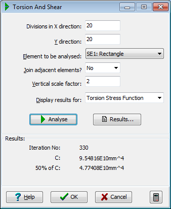
Note that the value of 'C' calculated and displayed by the program is not always suitable for direct incorporation as the section property for a grillage / frame analysis program. The value of 50% of 'C' is appropriate for some cases and is therefore also displayed. Some guidance on the interpretation of the torsional output is contained in the topic Interpretation of Torsion Results.
Form Graphic
Field Help
Divisions in x direction
Divisions in y direction
The number of divisions for the finite difference mesh must be entered for the x and y directions.
For sections whose overall dimensions fit into an approximately square shape, and which do not have a lot of details in them, the default values of 10 x 10 give a very good result.
For sections containing voids a finer grid may be needed.
For thin walled sections, the grid should be arranged so that a minimum of 3 grid points occur within the width of the material, (or 2 between the outside of a section and a void may suffice for torsion properties).
The solution time is approximately a function of the grid size squared. Although there is in theory no limit to the fineness of the grid, in practice the solution times can become exceedingly long, and in addition the program automatically adjusts the convergence for the iterative solution, so there is no benefit in having a finer mesh size than necessary.
Element to be analysed
The program allows you to select for analysis any of the individual elements that have been defined. The currently selected element is displayed in red.
Alternatively the currently selected element may be joined with any adjacent elements (refer next field).
Join adjacent elements
The currently selected element may be joined with any adjacent elements. Click in this field and set the entry to 'Yes' to join the elements, or 'No' to keep individual elements separate. In some cases (e.g. concrete U beam with slab on top) joining two elements may cause a void to be formed. Generally the program will generate this void and perform the appropriate analysis.
If the void is not generated, separate the elements (set the entry in this field to 'No') and try joining with the other element specified in the previous field.
Vertical scale factor
This field appears only when torsion analysis is selected. When the analysis has been performed and the shape of the membrane is displayed in the graphics window in isometric projection, the vertical scale of the membrane may be adjusted by increasing or decreasing the factor in this field. The membrane is redrawn immediately, so there is no need to change this field before the analysis is carried out.
Display results for
This field controls the calculations that are performed, and the graphics display. Click on this field to display a drop-down list. The options are:
| Item | Description |
|---|---|
| Shear Stress Function | The equivalent stress function for shear is most appropriately represented in contour form. The plot is calculated for a unit shear of 1kN applied parallel to the Y axis, and gives a visual indication of the shear flow in the section. |
| Shear Stress YZ | The shear stress YZ at any point in the section is related to the X- slope of the stress function membrane at that point. Selecting this option displays a contour plot of the slope of the stress function scaled such that it gives the YZ shear stresses in the current stress units that result from the 1kN unit shear described above. |
| Shear Stress XZ | The shear stress XZ at any point in the section is related to the Y- slope of the stress function membrane at that point. Selecting this option displays a contour plot of the slope of the stress function scaled such that it gives the XZ shear stresses in the current stress units that result from the 1kN unit shear described above. |
If any of the shear stress options are selected, the position of the shear centre is also plotted on the section.