Use Contour Plots to View MCT State Variables

MCT state variables are element output variables stored at every integration point within each element. To view MCT state variables in Patran, the bulk data file must first request that they be written to the output (.op2) file (see Request Output of the MCT State Variables). Refer to Appendix C for a complete description of each MCT state variable.

Contour plots are usually the most appropriate means of examining the distribution of the MCT state variables. To generate a contour plot with Patran, follow the steps below:

1. Click File > New and navigate to the directory containing the results. Name the database file and click OK.
2. Click File > Import and specify the Source as MSC.Nastran Input.
3. Navigate to the location of the bulk data file. Click Apply.
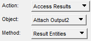
4. From the Analysis tab, set the Action to Access Results and set the Object to Attach Output2.
5. Click Select Results File... and navigate to the location of the .op2 file. Click OK.
6. Click Apply.

   

7. Click the Results button and on the Results tab select Create, Fringe.

   

8. Select a result to plot from the Select Fringe Result window and click Apply.

To view a contour plot of the MCT state variables, select one of the requested outputs (SV2, SV3, ..., etc.) from the Select Fringe Result window and click Apply. The number of SVs available to plot depends entirely on the number of state variables requested with the UDSESV entry.

The fundamental MCT state variable is SV2, which indicates the damage state of the composite material. SV2 is a real variable that can assume a finite number of discrete values between 1.0 and 4.0. The specific set of discrete values that SV2 can assume depends on the type of composite material (unidirectional or woven) and the specific set of material nonlinearity features used by Helius PFA during the finite element solution (see Appendix C). An MCT file (*.mct) is generated when an analysis is run using Helius PFA. This file contains the specific set of values that can be assumed by SV2 for each material in the model.

It should be noted that contour plots of fully-integrated elements can show values of SV2 that are less than 1 and greater than 4. This is entirely due to the scheme MSC Nastran uses to compute contour values. For element-based values, such as SV2, the computations vary depending on several criteria. In general, the extrapolation of integration point values to the nodal locations is the reason SV2 can be less than 1 and greater than 4 for fully-integrated elements.

Because SV2 is a discrete real value between 1 and 4, it is important to change the contour plot settings so that a unique color contour is associated with each discrete integer value of SV2. In the case where SV2 can assume values of 1.0, 2.0, or 3.0, set the color spectrum to include just three colors and modify the range of values associated with each color.

1. First, set the color palette by clicking Display > Spectrums...
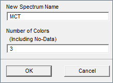
2. Click the Create button and give the new spectrum a name and set the number of colors to 3 as shown below.

   

3. Now assign the red, green, and blue colors to the spectrum as shown below on the Spectrums tab.

   

4. The next step is to define a range. Click Display > Ranges... and create a new range in the window that appears.
5. Give the range a name, set the Data Methods Algorithm to Manual, and set the Manual Aids to None.
6. Set the Number of Sub-ranges to 2 and check on the To box in the Label Display window.
7. Now define the range as shown below.

   

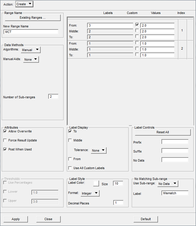
   The blue color is now associated with SV2 = 1.0, green with SV2 = 2.0, and red with SV2 = 3.0.

8. Finally, set the Action to Assign to Viewport and click Apply.

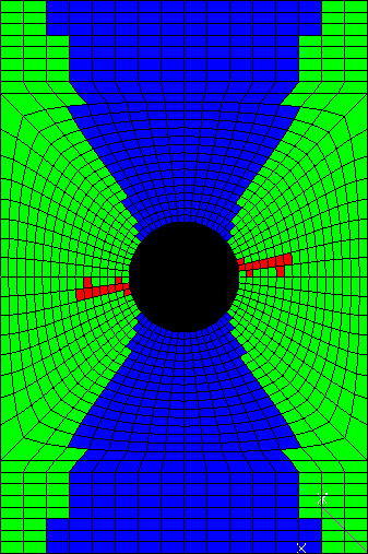
The image below shows a contour fringe plot of SV2 for an axially loaded composite plate with a central hole. The use of three discrete colors makes it easy to identify the regions where each discrete composite damage state occurs. The blue elements (SV2 = 1) are undamaged, the green elements (SV2 = 2) have failed matrix constituents and undamaged fibers, and the red elements (SV2 = 3) have failed matrix and fiber constituents. In this plot, the element averaging domain has been set to None, so that each element retains its value at the element nodes.

The remaining MCT state variables (>SV2) are continuous real variables. Therefore, it is not critical to manage the number of color contours when plotting.

Selection of Section Points

When viewing finite element solution results for laminated composite structures, you must be aware of the numbering of section points through the thickness of multilayer elements. A contour plot will only use the values of the variable stored at a particular section point. Therefore, to view a contour plot for a specific material layer, you must choose a section point that lies within that material layer. To choose a specific section point, click the Position button on the Select Results page of the Results tab. Choose the section point of interest from the available layers. You may also create an envelope plot by selecting Maximum, Minimum, Average, Sum, or Merge from the Option menu.

As an example of the recommendations above, consider the image below. This shows contour plots of SV2=1,2,3 at several points in time during a progressive failure analysis of a composite plate with a central hole. The plate has eight material plies and is loaded in tension. Since these contour plots are envelope plots (Option = Maximum), the color at any location represents the highest value of SV2 achieved at any of the section points distributed through the thickness of the 8-ply laminate. In these plots, blue elements have no failure at any of the section points distributed through the laminate thickness. The green elements have at least one section point where matrix failure has occurred, while the red elements have at least one section point where both matrix and fiber failure occurred.

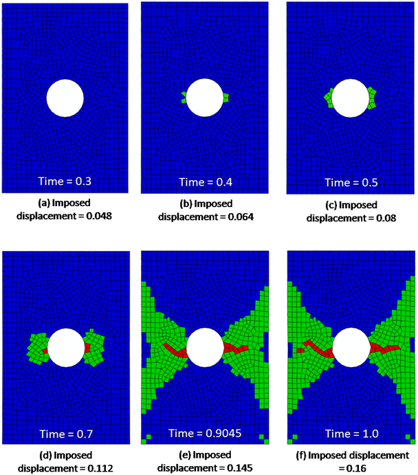
Several important observations can be made regarding the sequence of envelope contour plots shown above (Averaging Domain = None):

• At time = 0.3, every element is blue, meaning no points in the composite plate have experienced any type of failure.
• At time = 0.4 there are some green elements at the edges of the hole. Within these green elements, at least one material ply has experienced a matrix constituent failure. However, the plot does not specify which of the material plies have experienced a matrix constituent failure.
• Comparing the plots at times 0.4 and 0.5 indicates the progression of matrix constituent failure as the load increases.
• At time = 0.7, the matrix failure has spread further, and there are three elements with fiber failure, as indicated by the red elements. Again, the red elements indicate that at least one of the 8 material plies has experienced a fiber constituent failure.
• At time = 0.9045, there is significant matrix failure, and the fiber failure has spread out towards the plate edges.
• At time = 1.0, there is additional matrix and fiber failure.

Note: When examining results for large models with Patran, MSC Nastran requires the following environment variable setting:

>>SET DRANAS_NAST_MEM=2048MB

Consult the MSC Nastran Quick Reference Guide for further details.