These techniques can be applied to nearly all electronics applications, independent of the physical configuration. These sections are referenced throughout the application-specific sections.

Sheet Metal

Sheet Metal parts are prevalent in many electronics assemblies. To improve modeling efficiency, sheet metal parts should be simplified or removed. Some basic guidelines include:

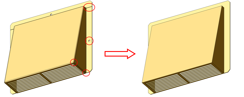
• Suppress all fasteners and related holes unless they are critical to the heat flow path.
• Remove rip corners and bend reliefs
• Change the bend radius to 0 to create sharp corners.
• Remove gaps where tabs overlap.
• Replace perforation patterns with simple geometry and a distributed region:

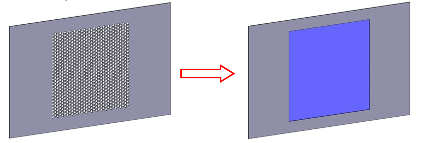
• An example of a simplified sheet metal part:

• In most cases, sheet metal parts built with CAD sheet metal design features and design tables are not recommended.
  • Sheet metal features such as corner features and bend radii cannot be removed and often cause the mesh size to be too large. This can lead to significantly longer analysis times, and reduced solution efficiency.
  • The recommended approach is to build sheet metal parts as solid features in CAD. Omit detail that is not relevant to the flow and thermal simulation.

Creating the Flow Volume

In many of the configurations described below, an air volume is constructed around the device.

There are two primary ways to create the surrounding flow volume:

• Build it in the CAD model.
  • If the fixture must contact a surface of the region, this is the recommended approach.
  • A good technique is to create a cavity that surrounds the fixture. This region will be filled automatically when the model is launched, and will be meshed. It serves as a mesh refinement region, and because it eliminates the interference between the fixture and the surrounding air volume, the part names will not be modified.
• Use the External Volume Geometry tool in Autodesk® CFD.
  • This eliminates the need to add an "Air" part to the CAD model.
  • Note that this technique should not be used if the fixture must contact a side of the air volume (as in the Wall-Mounted configuration).

A useful technique that can reduce the model size and analysis time is to take advantage of symmetry. If the device is half- or even quarter-symmetric, the overall model size can be reduced significantly. For more about symmetry.

Material Devices

Use material devices to simulate components often used in electronic devices. These provide an efficient way to simulate the effect of the physical device, without adding complexity to the mesh and analysis model.

• To simulate a screen or baffle, use a distributed resistance material.
• To simulate a printed circuit board, use a printed circuit board material.
• To simulate an axial fan, use an internal fan material.
• To simulate a Compact Thermal Model, use a CTM material.
• To simulate a Thermo Electric Device, use a TEC material.
• To simulate a heat exchanger, use a Heat Exchanger material.

Heat sinks and heat pipes can also be simulated using simple geometry after the flow and thermal performance are characterized.

An Alternative way to simulate air in thin gaps and regions using a "Solid Air" material

For very thin enclosures, the heat transfer is largely dominated by thermal conduction instead of convection. In certain applications, it is possible to accurately simulate the heat transfer without having to solve for the flow. The advantages of this are significant:

• Faster analyses: Because only conduction is computed in the gap, one equation is solved per iteration instead of five. (In the standard approach, both conduction and convection are computed per iteration.)
• Smaller simulation models: The mesh is smaller because Wall Layers are not created in solids.
• Consistent accuracy with the true natural convection solution, when used appropriately.
• Mesh-independent thermal solutions are often easier to achieve than mesh-independent flow solutions

Applications

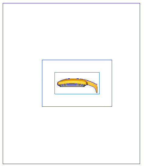
This technique can be used for devices with thin enclosures or for focused simulations based on thin gaps between components. Examples include:

• Routers
• Space between two circuit cards
• Space between a housing and a PCB
• Space between sheet metal divider and a PCB

Modeling Strategy

A solid material with the thermal properties of air is included in the Default material database. This material is called Solid Air. Select it from the list of solid materials in the Materials quick edit dialog.

Running

• Flow = On

• If the component temperatures are relatively high, Radiation = On (Radiation often has a stabilizing effect. In some models, neglecting the effects of radiation produces temperatures roughly 20% higher than actual values.) A useful strategy is to run 200 iterations without radiation, and then enable radiation and continue. This reduces the analysis time, and provides insight into the effects of radiation. Be sure to specify appropriate emissivity material property values. For more about modeling radiation.

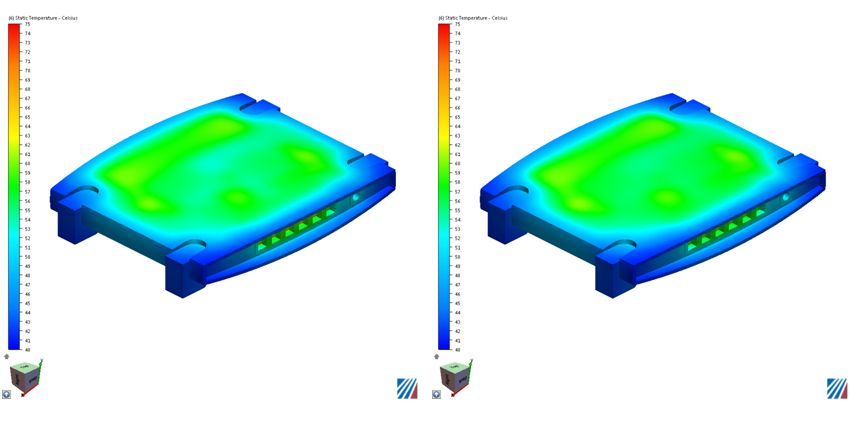
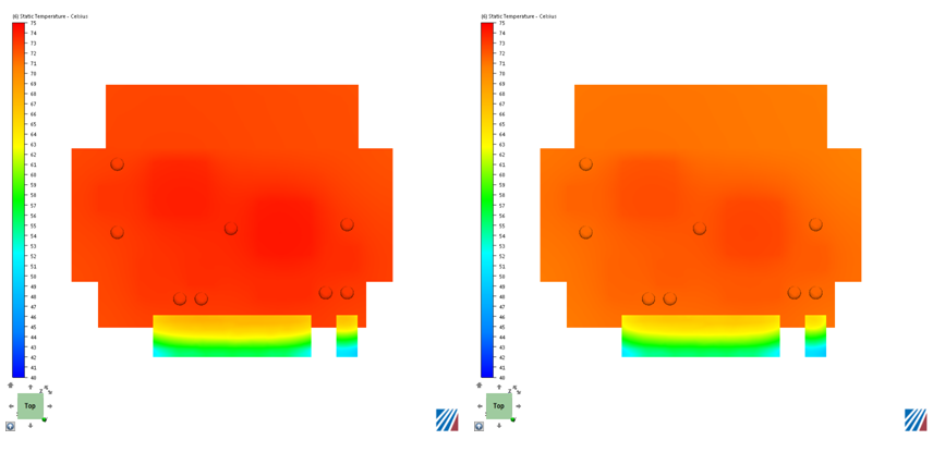
Example Results

The images on the left show temperature from a flow and thermal analysis. The images on the right show temperatures from a "solid-air" analysis:

When is this approach Valid?

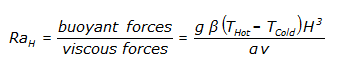
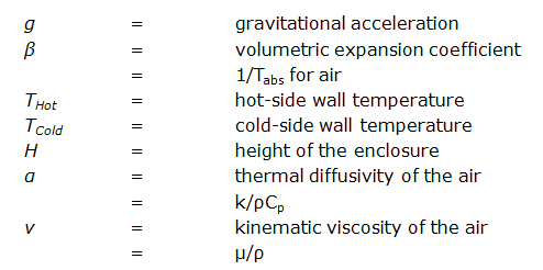
The Rayleigh number describes the transition point. Qualitatively, the Rayleigh number is the ratio between buoyant forces and viscous forces. The buoyant forces cause air motion; the viscous forces oppose it. The Rayleigh number is computed from:

The transition from conduction to convection, the critical Rayleigh number, has been determined to be:

• Horizontal: Ra(critical) = 1708
• Vertical: Ra(critical) = 1000

Example:

An electronics system has a ten degree differential, and the following parameters:

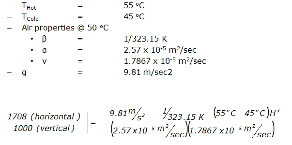
The resultant critical thickness values are:

• Horizontal: H = 13.7 mm
• Vertical: H = 11.5 mm

For a ten degree temperature differential, the air in a horizontal enclosure that is 13.7 mm thick or less (or a vertical enclosure that is 11.5 mm thick or less) can be modeled as a solid with the same properties of air.

Computing the Critical Gap for at other temperature differentials

The Rayleigh number definition can be used to show that the temperature differential is proportional to the gap cubed. Using the values computed for a 10 degree differential, it is easy to compute the gap at a different temperature differential using the following:

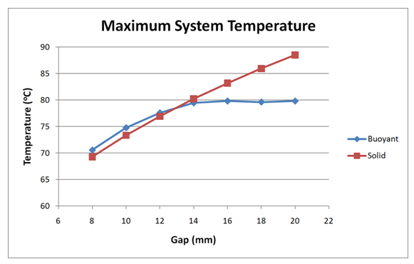
Accuracy Study

To assess the accuracy of this approach, a study was performed in which the gap was varied from 8 to 20 mm, and run with both methods. Below the critical gap, the agreement between buoyancy and "solid" air is quite good. Above the critical gap, as expected, the agreement degrades due to the increased role of convection as a mode of heat transfer:

Meshing Strategies

Focus the mesh in the region so that the geometric detail of the device is modeled and the flow and thermal gradients around the fixture are represented numerically.

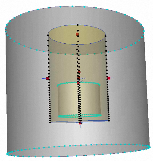
An extension of this technique is to nest multiple regions around the device. Create these regions in the CAD model as Refinement Regions in the Autodesk® CFD Mesh task do not support this technique. This concept is illustrated:

The mesh distribution in the inner-most region is the finest, and focuses the mesh where the gradients are highest. Because this region is small relative to the calculation domain, this high-density mesh does not propagate far, which keeps the overall mesh count from getting too big. The mesh distribution in the second nested region is a little more coarse, and the mesh in the remainder of the domain is even coarser. This approach efficiently concentrates elements only where they are most needed, providing an efficient use of meshing and solving resources.