Activity 2: Simplify model 1 and apply thermal loads

In this activity, you remove model components that are extraneous to the thermal analysis, and then apply thermal loads to simulate the heat transfers across the radiator.

You assume that the inner wall of the pipe is the same temperature as the water that is flowing it. You also assume that the flow rate is high enough that the temperature change of the water is negligible across the radiator. The fins, however, will lose heat to the environment by natural convection and by radiation.

In this activity, you

Remove model components that have no influence on the simulation, to reduce the analysis time
Apply a thermal load to the interior faces of the pipe, to represent the heat from the 75 C water flowing through them
Apply a thermal load to the fins to represent the heat radiating from the hot pipe through the fins and into the environment
Apply a thermal load to the fins to represent heat loss, by convection, to the environment
Automatically detect the contact sets and use the default settings.

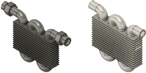
Radiator model before modification (left). Radiator model, simplified, with thermal loads applied (right).

Prerequisites

Activity 1 is complete.

Steps

Remove the fittings and the water volume components, because they do not influence the simulation, but they do contribute to the analysis time.

Note: Simulation computing time is heavily dependent on the mesh. You remove unnecessary objects to prevent them from being meshed and included in the simulation.
1. Click (Simulation workspace > Setup tab > Simplify panel > Simplify), to access the Simplify environment.
2. In the Browser, expand Model Components.
3. Right-click the Water:1 component, and select Remove. Notice, the Remove action is added to the Simplify Timeline at the bottom of the canvas.
  Note: Remove deletes the part from the Simulation model, but has no effect on the geometry in the Design workspace.
4. Repeat step c to remove the Fittings:1 component.
5. Click Home View next to the ViewCube to return the model to its original size and orientation.
6. Click (Simulation workspace > Simplify Solid tab > Finish Simplify panel > Finish Simplify) to return to the Setup tab.
  Note: The Timeline has changed and no longer shows the Remove actions. These actions are visible only on the Simplify Timeline.
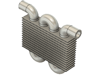
Open the Thermal Loads dialog and select all 24 faces of the pipe.
1. If necessary, in the Browser, expand Model Components.
2. Click next to Fins to hide them.
3. Click the RIGHT face of the ViewCube to adjust the orientation of the pipe.
4. Click (Simulation workspace > Setup tab > Loads panel > Thermal Loads, to open the Thermal Loads dialog.
5. In the Thermal Loads dialog, confirm that the Load Type is Applied Temperature.
  Tip: The software prevents you from putting incompatible loads on the same surface. Specify the load type before selecting the Object Type.
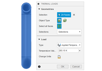
6. Click Select all faces so you can select all of the pipe surfaces, then click on the pipe.
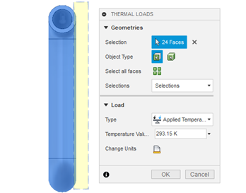
Deselect the outer faces of the pipe, so that the thermal load is applied only to the inner faces of the pipe.
1. In the Thermal Loads dialog, click Select all faces to deactivate it so that you can use standard selection to deselect the exterior faces of the pipe.
2. Left-click to the right and above the model and drag a window selection over the edges on the right side of the model.
  Note: It is important to pull the selection window to the left to properly deselect surfaces.
Apply a thermal load of 75 C to the inside faces of the pipe.
1. In the Thermal Loads dialog, click Change Units.
2. Select C from the drop-down list.
3. Change the Temperature Value to 75 C.
  Note: The temperature actually depends on the water heater or boiler. It is always a good idea to make a conservative assumption.
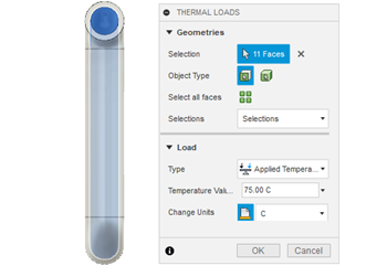
4. Click OK to accept the temperature and close the dialog.
Confirm that the correct temperature has been applied to the correct pipe faces.
1. In the Browser, expand Load Case1, then expand Loads.
2. Hover over Applied Temperature1, then click Edit. The applied temperature is shown and the 11 inside faces are highlighted in blue.
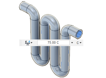
3. Click Cancel to close the Thermal Loads dialog.
Apply a thermal load to the fins to simulate loss of heat to the environment by Radiation, at ambient temperature.
1. In the Browser, under Model Components, click next to Fins to make them visible.
2. Click next to Pipe to hide it.
3. If the orientation was changed, click the RIGHT face of the ViewCube.
4. Click (Simulation workspace > Setup tab > Loads panel > Thermal Loads, to open the Thermal Loads dialog.
5. In the Thermal Loads dialog, change the Load Type to Radiation.
6. Left-click and drag a window around all the fins, and confirm that 140 Faces are selected.
7. Click the down arrow directly above the ViewCube, to change the orientation, so the top of the fins is pointing out of the canvas towards you.
8. Left-click on the model face to the left and above the top hole in the fins and drag a window selection over all the holes. Notice that now only 84 Faces are selected.
  Note: It is important to pull the selection window to the right to properly deselect only the surfaces that are fully enclosed by the window.
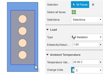
9. Leave the default values for Emissivity 1 and Ambient Temperature Value 293.15 K (20 C), then click OK to apply the command and close the dialog.
Apply a thermal load to the fins to simulate loss of heat to the environment by natural convection, at ambient temperature.
1. Click the RIGHT face of the ViewCube, so you can see all the fins again.
2. Click (Simulation workspace > Setup tab > Loads panel > Thermal Loads, to open the Thermal Loads dialog.
3. In the Thermal Loads dialog, change the Load Type to Convection.
4. Left-click and drag a window around all the fins, and confirm that 140 Faces are selected.
5. Click the down arrow directly above the ViewCube, to change the orientation, so the top of the fins is pointing out of the canvas towards you.
6. Left-click on the model face to the left and above the top hole in the fins and drag a window selection over all the holes, to select the same surfaces as in the previous step.
7. Leave the temperature at ambient, and change the Convection Value to 5 W /(m^2 K).
  The ambient reference should be the same or the loads will fight each other.
8. Click OK to apply the command and close the dialog.
  
  Tip: Check the Browser to confirm all three loads are shown. Confirm that the thermal loads on the fins are correct, in the same manner as you confirmed the pipe.
Define the contacts between the bodies that makeup the model.
1. Click (Simulation workspace > Setup tab > Contacts panel > Automatic Contacts, to open the Automatic Contacts dialog.
2. Click Generate to accept the command and close the dialog.
  The parts are all coincident so the default tolerance is acceptable.
3. In the Browser, click next to Pipe to make it visible.
4. Click Home view above the ViewCube to return the model to its original size and orientation.

Activity 2 summary

In this activity, you simplified your model to reduce your analysis time, and applied thermal loads to the radiator pipe and fins:

Removed model components that have no influence on the simulation, to reduce the analysis time
Applied a thermal load to the interior faces of the pipe, to represent the heat from the 75 C water flowing through them
Applied a thermal load to the fins to represent the heat radiating from the hot pipe through the fins and into the environment
Applied a thermal load to the fins to represent heat loss, by convection, to the environment.
Automatically detected the contact sets and used the default settings.