
Introductory remarks:
Loads, in great majority, originate from the gravity (masses). Thus dynamic calculation needs these masses to be taken into account. To enable the user an easy conversion of static loads (gravity loads) into masses the special command "MASses ACTive" was applied into text file analyzer.
This will allow the users to define load only once for the purpose of static analysis and then to use them to create mass distribution over the computational model of the structure to perform any dynamic analysis.
Command needs two elements to successful conversion. The first is the set of directions in which masses are be active. Usually all global directions (X, Y, Z) are used, because only in specific calculations inertia acts not on all of them. The second is the inertia magnitude. This is defined by the static load case number, and the direction of the loads, which are be taken into account during conversion. Additionally, an extra coefficient may be given to multiply the load value.
The character of the load is automatically transformed into the masses: concentrated forces are transformed into concentrated masses, moments - into rotational inertia, distributed forces - into continuous masses.
Syntax:
ANA [ DYN | MOD | TRAN | HAR | SEIsmic | SPEctral ],( concerns all the dynamic analysis types)
CASe (#<number> <name>)
MASess ACTive [X/Y/Z]
[X|Y|Z ] (MINus|PLus) <case_list> COEfficient=<c>
General principles:
Let r = r(x) be a function of the mass density distribution within given element while N(x) be the nodal interpolating function matrix (shape function matrix). As a base of further treatment consistent mass matrix of an element will be created according to the following general formula (1) :
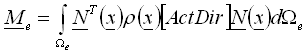 , (1)
, (1)
where:
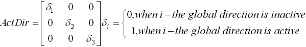
The global direction activity flags are set by MASess ACTive [X/Y/Z], i.e. any direction is active if specified. This is the consequence of generalRobot style of the mass treatment, where some components of inertia forces may be neglected during the analysis.
Mass matrix will be created from all the loads belonging to all load cases specified in <case_list> acting on current element/node according to the following rules:
- Each load record from specified case is converted to the mass separately and independently from other loads and masses.
- Only simple load cases (no combinations !) may appear on the list (but in one dynamic case the list of static cases may be given to be converted into masses).
- Total mass matrix is created as a sum of mass matrices from all above load components and from predefined mass due to dead weight of the structure and/or specified element masses. Thus also part of a mass matrix originated from loads will be submitted to diagonalization and/or negligence of rotational inertia part if specified by COH|CON, ROT setting .
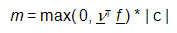
- The value of the density function in given point is created as the value of the projection of the current force vector f on the vector n of uniquely and obligatorily specified global direction
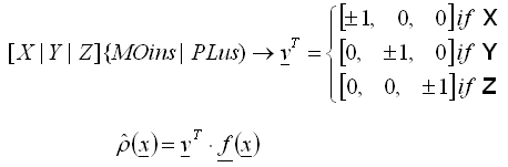 , (2)
, (2) - Only positive values are taken into account in each integration point, thus
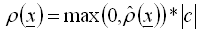 , (3) Note: Above rules are intended to allow an easy selection of loads originated from gravity. As nothing like default gravity direction exists, signed direction specification must be done by the user.
 - All directions used to define load to mass conversion must be acceptable for current general structure type, thus PLAte accepts only Z direction, for other plane types only X and Y will be accepted. Incompatible direction specifications will be ignored or error will be reported. 3D structural types accepts all global directions.
Example:
Consider a beam, loaded centrally by the gravity load Fy= - 120 kN. Let the static case shown below has a number 3. To calculate free vibration modes of this structure in the case number 10, taking into account this mass (Fx=Fy= 12 232 kg) one can use the following command:
ANA MOD=3 MAS=CON
CAS #10 modal
MASses ACTive X Y
Y MINus 3
Details of conversion for different load types
Loads acting on beam elements
- uniform element load
[Px=<px.>/Py=<py>/Pz=<pz>] (LOCal/GLObal) (PROjected) ([R=<r>])([R=<r>])
The load density vector is transformed to global directions as specified by setting :
(LOCal/GLObal) (PROjected) ([R=<r>]), taking into account (PROjected) flag as for load treatment, then uniform mass distribution is set according to (2) (3)
- dead load
Dead load is converted to mass equivalently to the uniform element load
Note: This operation should be used with caution, as mass originated from dead load of the structure is taken into dynamic calculations automatically (if only material density is greater than 0) - variable element load
(X=<x1>)[ P=<p1>] ((JUSque)(X =<x2>)[P=<p2>] ) (R=<r>) (LOCal/GLObal) (RELative) (PROjected)
load is transformed to global directions as specified by setting :
(LOCal/GLObal) (PROjected) ([R=<r>])
then uniform mass distribution is set according to (2)(3)
Note: Rule (3) implicate the following treatment of variable sign load, for each load record (component) separately (not for the total load being the sum of all loads acting on given element), as shown in Fig.1. Fig.1
Fig.1 - concentrated element force
[X=<x>] [F=<f>](R=<r>) (Local)(RELative)
The total mass m concentrated in a point x 0 is evaluated from global representation of force vector f as follows:
 , (4)
, (4) Consistent mass matrix is then evaluated, as if mass distribution would be represented by Dirac's delta function leading to:
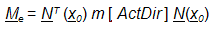 , (5)
, (5) - concentrated element moment
[X=<x>] [F=<fc>] (R=<r>) (LOCal)(RELative)
As mass direction specification does not concern directions of rotational inertia, thus separate rule should be established to perform the conversion between concentrated element moment and rotational inertia of a certain body attached to the element.
Vector style transformation of <fc> is performed according to (R=<r>) (LOCal) settings to obtain a vector I referred to element local co-ordinate system. To omit necessity of inconsistent vector style transformation (while tensorial one should be used), load should be given as LOCal and no R=<r>, otherwise the warning will be issued .
There is assumed that element local co-ordinates coincide with principal axis of inertia of the body, thus
 represent principal inertia moments in element local co-ordinates. From this results the following modeling limitation:
Fig. 2
Correct situation
Incorrect situation, modeling impossible
- distributed element moment
[M=<m>] (LOCal)
In this definition, <m> is a vector, which, after vectorial style transformation to element local co-ordinate system, represents densities of rotational inertia referred to element local axis per element length.
All notions as for concentrated element moment, (see Fig. 2), holds.
Loads acting on surface elements
- uniform element load
[Px=<px.>/Py=<py>/Pz=<pz>]
Load density vector is evaluated, then transformed to mass density according to (2)(3)
- dead load
Dead load is converted to equivalent uniform load and further treatment as above
Note: This operation should be used with caution, as mass originated from dead load of the structure is taken into dynamic calculations automatically (if only material density is greater than 0) - variable element load
[P=<p1>] AU <n1>( [P=<p2>AU<n2> ([P=<p3> AU<n3>))
In each integration point load density is evaluated, then transformed to mass density according to (2)(3), see Fig. (1). Enhanced integration rules are used with
NGAUS = 3x3 for Q8,
= 7 for T6,
= 2x2 for Q4
= 3 for T3
- variable load inside a contour
[P=<p1>] AU <n1>( [P=<p2>AU<n2> ([P=<p3> AU<n3>)) PROjected DIRection <v> _CONtour <l_node>
In each integration point load density is evaluated, then transformed to mass density according to (2)(3), see Fig. (1). In the case when not whole area of the element belongs to the contour, fully automatic integration over the up to 100x100 point mesh is performed within element, to reach required accuracy of integration. Thus using this option may sometimes slow down the mass matrix evaluation process.
- variable load along the line
LIN
<n1>[P=<p1>] Jusque <n2> (P=<p2>) ( [LOCal (GAMma=<gamma>)] )
Only translational force may be converted to element mass distributed along the line.
3-point Gauss type integration rule is used on each in segment of the line crossing the element. In each integration, load density vector is transformed to global co-ordinate system, then treated according to (2)(3) to evaluate mass distribution along the line.
- concentrated load on auxiliary point
NODe (auxiliary)
F=<f> ( [R=<r>] )
Only translational force may be converted to element mass ( for beam elements moment - rotational inertia conversion was allowed, here is prohibited). Force vector <f> is transformed if necessary to global co-ordinate system and then treated according to (2),( 3) to evaluate the mass value attached to the point within the element, then the mass matrix is evaluated using (5). The element to which mass will be attached is searched automatically.
Nodal loads
- concentrated force
NODe
F=<f> ( [R=<r>] )
Force vector <f> treated according to (2)(3) to evaluate the nodal mass value
- concentrated moment
NODe
F=<c> ( [R=<r>] )
As mass direction specification does not concern directions of rotational inertia, thus separate rule should be established to perform the conversion between concentrated nodal moment and rotational inertia of a certain body attached to the node.
Vector style transformation of <fc> is performed according to (R=<r>) setting to obtain a vector
 referred to global co-ordinate system. To omit necessity of inconsistent vector style transformation (while tensorial one should be used ), no LOCal should be given as and no R=<r>, otherwise the warning will be issued.
 There is assumed that global co-ordinates coincide with principal axis of inertia of the body, thus
represent principal inertia moments in global local co-ordinates. Note: This rule is different than those used in case of concentrated mass attached to beam element.