
7.4 Dead Load & Diff Temp Load on a Finite Element Slab
Subjects Covered
- Dead loads in FE
- Differential temperature in an FE Slab
- The use of composite members to represent FE results
- FE results with discontinuities in slab thickness
- Principle moment vectors
Outline
Consider the finite element slab, as described and modelled in example 6.5 which has variable thickness and a curved profile in plan.

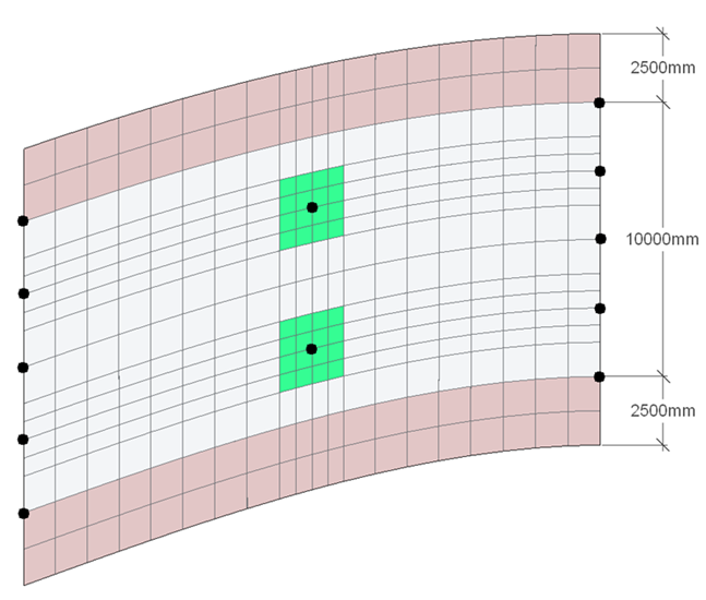
It is required to establish the distribution of load to the supports due to its own self weight and to examine the load path by considering principle moment vector plots. The load will be based on a weight density of reinforced concrete of 25kN/m³.
It is also required to consider the effects of an applied temperature profile through the thickness of the slab, in accordance with EN 1991-1-5, with respect to the secondary moment created. Only positive differential temperature will be considered and it is assumed that a surface thickness of 100mm will be applied.
The temperature load will be applied as a combination of a temperature gradient load and a general temperature rise. The values of these two components will be different for the variable thickness of slab. For the purpose of this example we will only consider the main slab of 500mm and the cantilever slab of 300mm. The effects on the column head will be assumed to be that of the 500mm slab.
The two values of temperature required here can be calculated from first principles using the expressions:
 for temperature gradients,
and
 for membrane temperature.
E is the elastic modulus of the concrete (35.2205kN/mm²), I and A are the moment of inertia and the area of a 1m section of the slab and is the coefficient of thermal expansion (1.0E-5).
M and F are the restraining Moments and Forces obtained when applying the temperature profile to a 1m wide section of the slab. These can be obtained by carrying out a simple differential temperature analysis (using Autodesk Structural Bridge Design) of 1m wide sections of the two thicknesses of slab, by following the procedure in example 3.3. The results of this and a section property analysis are as follows:
500mm thick slab
| I = 1.0417E10mm⁴ | A = 5.0E5mm² | |
| M = 72.63kNm | F = 534.91kN | giving |
| Tg = 19.8ᴼ/m | Tₘ = 3.03ᴼ |
300mm thick slab
| I = 0.225E10mm⁴ | A = 3.0E5mm² | |
| M = 23.75kNm | F = 287.04kN | giving |
| Tg = 29.97ᴼ/m | Tₘ = 2.72ᴼ |
Procedure
- Start the program and use the Home Open button to open the file “My EU Example 6_5.sst” created in example 6.5. Close the Project Overview with the ✓ Done button.
- Using the File | Titles menu option, change the title sub title of the example to “Example 7.4” Change the Job Number: to “7.4” and put your initials in the Calculations by: field before closing the form in the normal way.
Dead Load
Click on Structure Loads at the bottom of the navigation window and then click on + at the top of the window and select Finite Element Load | External Load from the dropdown list.
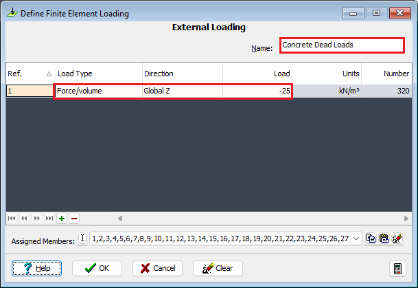
In the Define Finite Element Loading form, insert a new row using the table + button, and set Load Type to “Force/volume”, Direction to “Global Z” and Load to “-25”.
Window around the complete structure in the graphics window to select all the elements. It doesn't matter that they have different thicknesses as the load applied is a volume load.
Set Name: to “Concrete Dead Loads” before closing the form with the ✓ OK button.
Temperature Load
Click on at the top of the navigation window and select Finite Element Load | Temperature Load from the dropdown list.
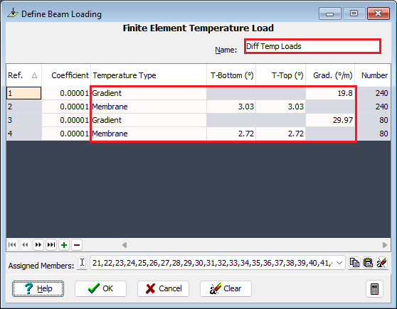
In the Define Finite Element Loading form, insert a new row using the table + button, and set Temperature Type to “Gradient” and Grad to “19.8”. The default Coefficient is correct.
This temperature gradient needs to be applied to the 500mm and 700mm thick slab. To do this click on the filter button
 in the graphics window toolbar, click on the De-select all Selection Tasks, and then set Select By: to “Structure Property”. Move the 500mm and 700mm slab properties into the Selected Groups: field using the “>” button and then close the Member Selection Filter form with the ✓ OK button.
Window round the complete structure in the graphics window to select these elements.
Add a second row to the table and set Temperature Type to “Membrane” and TBottom to “3.03”, press Enter. Window round the complete filtered structure again to apply this to the 500mm and 700mm thick elements.
Add a third row to the table and set Temperature Type to “Gradient” and Grad to “29.97”. This time the 300mm thick elements must be selected.
Use the filter tools in the same way as 9 above to filter the 300mm thick elements only and then window round the entire structure.
Add a fourth row to the table and set Temperature Type to “Membrane” and TBottom to “2.72” then press Enter. Window round the complete filtered structure again to apply this to the 300mm thick elements.
Change the load case Name: to “Diff Temp Loads” before closing the loading form with the ✓ OK button.
Analysis
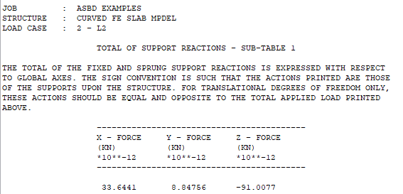
Use the menu item Calculate | Analyse Structure to perform the analysis and then click on the Analysis log file icon on the Analysis form to open the log file.
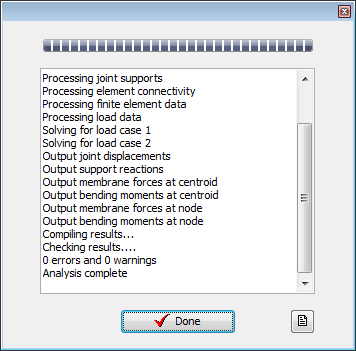
Check in the displayed text file that the total load applied is equal and opposite to the total reaction for the Dead Load case. Note that the total reaction for the Thermal load case, L2, is zero (or very close to zero) because temperature loads are internal loads.
Close the log file then close the Analysis form with the ✓ Done button.
Results – Dead Load Case
Use the main menu File | Results to open the results viewer. Set the view to be combined graphic and table, as shown below, by using the menu items View | Set Default Layout | Graphic Above Table. Adjust window size to suit by holding the left mouse button down on the dividing line between the graphics and table and dragging to a new position.
In the dark blue area at the top of the window (Results Controller) set Results For: to “Joint”, Name: to “L1: Concrete Dead Loads” and Effect: to “Support Reactions”.
In the graphics toolbar, the Results For: field should be set to “FZ”
Change the viewing direction to isometric by clicking on the Graphics toolbar icon
 and then annotate the results using the orange General Button on the right of the graphics window. Use the “Format” button next to the Results tick box and ensure Display All values is selected and SOP: is set to “Result” before closing the Format (Text Setup) window with the ✓ OK button. It may be necessary to click on the “Auto Redraw” button on the graphics toolbar to show the results.
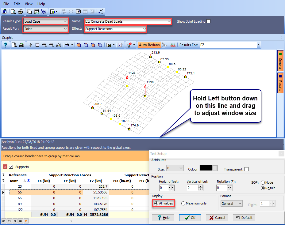
The distribution of dead load to the supports can be clearly seen.
To display how this load gets to the supports we can view the moment load path by plotting the principal bending results.
Change the results annotation to Maximums only and then set the fields in the Results Controller to those shown below. The Results For field in the graphics toolbar should be set to “Principal Values – Maximum” to show a faded contour plot together with two lines at the centroid of the element indicating the relative magnitude and direction of the principal moments. Click on Auto Redraw if the graphics view is not automatically automated.
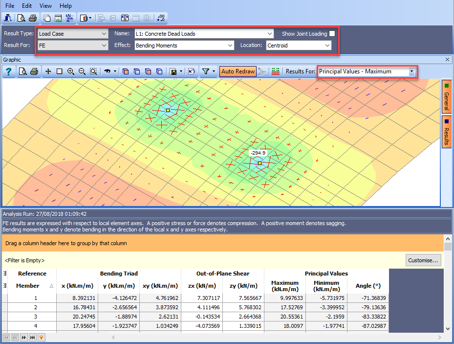
Red lines represent hogging moments and blue lines represent sagging.
To graphically represent the bending moment in the longitudinal direction, for the dead load case, the Results Controller fields need to be set as shown below and the Results For field in the graphics toolbar should be set to “Bending Triad –x”.
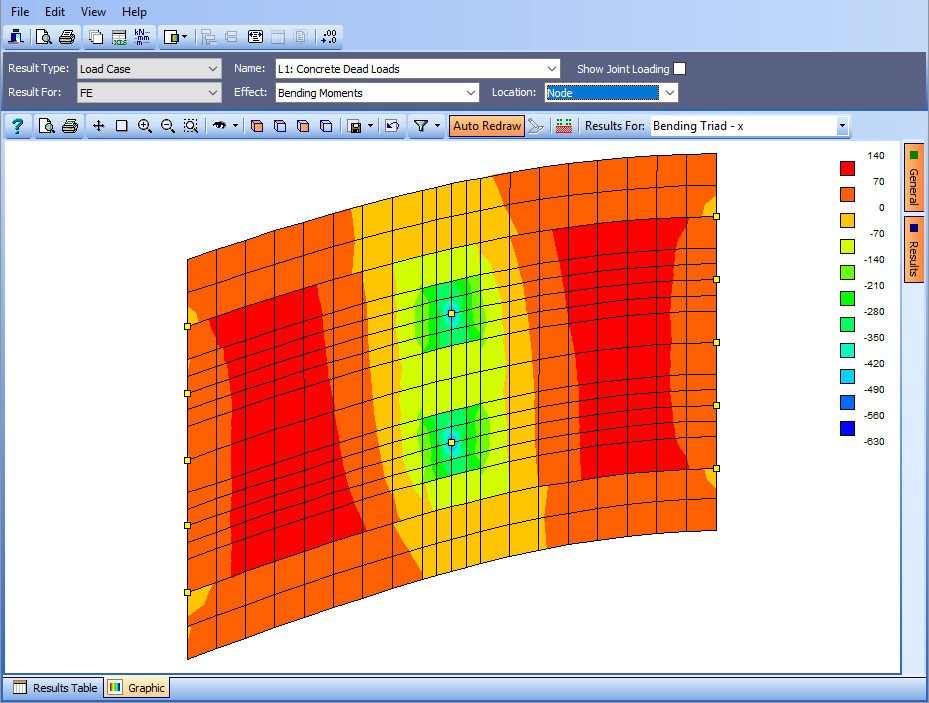
The view shown here has been changed to a Tabbed view (using the View menu) and the viewing direction set to plan view. There are two significant points to note here.
- The x moment values are per m width and represent bending in the local xz plane. For this structure the default local x axis is the same as the global X axis. If we wanted to change this such that the local x axis was in the direction of the deck centre line we would need to change them by adding an Advanced FE Set | Local Axes item to the “Structure” Navigation Window to align them to the design line. The load cases would need resolving before viewing the results.
- The Location: field in the results controller is set to “Node” rather than centroid or nodal averaged results so that the discontinuity along the boundary between the two slab thicknesses is represented.
Close the Results viewer.
Results – Differential Temperature Load Case
The secondary moment results caused by the differential temperature case are best displayed as bending moments on a virtual beam strip, the width of two narrow elements, passing over the lower of the mid span supports. The results are to be integrated over the width of this beam strip. To do this in Autodesk Structural Bridge Design we use the concept of a “Virtual Member”.
To define this Virtual Member we click on the menu item Calculate | Define Virtual Member.
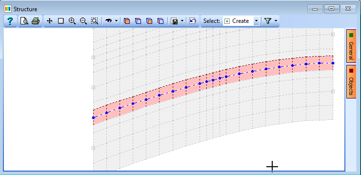
The elements that make up the virtual member are then selected graphically by first setting the Pick Mode: to “Finite Element” and then clicking on the elements one by one – as shown below.
The Reference Axis is defined by setting the Pick Mode: to Node and then clicking on the nodes, one by one, along the centre of the virtual beam from one end to the other.
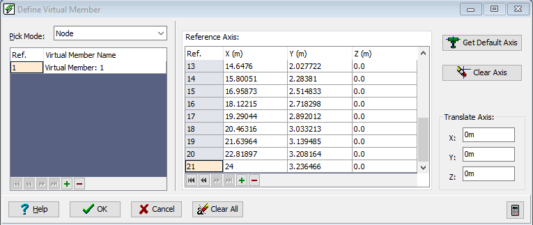
Close the Define Virtual Member form with the ✓ OK button.
Open the Results viewer and set the fields in the dark blue Results Controller area to those shown below. The viewing direction has been set to a south elevation.
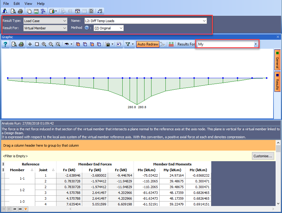
This now shows the bending results of a beam strip 1.25m wide with its centre line along the virtual member axis.
The results are obtained by integrating the FE results across the beam strip and resolving them at each of the axis points. There are two integration/ resolving algorithms that can be used, Method 1 and Method 2 and it is up to the user as to which is the most suitable. The method is selected in the results controller. The basic suitability criteria can be displayed by clicking on the small, circular “?” button next to the Method radio buttons. Selecting Method 3 will display the enveloped results of Method 1 and Method 2.
In our case method 2 has been selected as most suitable. If in doubt, use the most conservative approach.
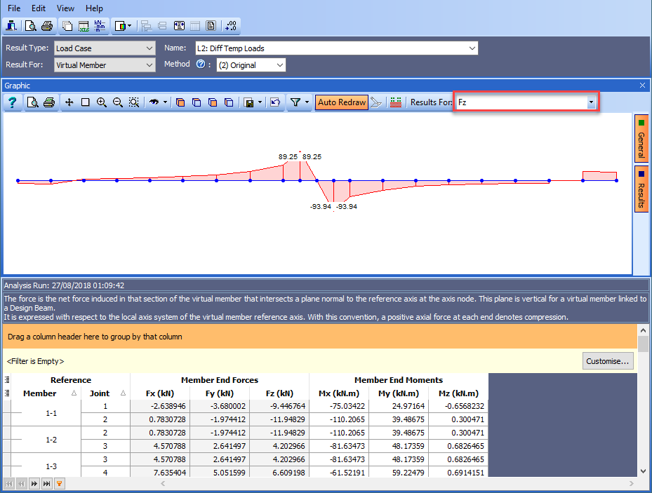
Shear results can be displayed in exactly the same way.
Close the results viewer.
Use the main menu File | Save As to save the data file with a name of “My EU Example 7_4.sst”.
Close the program.
Summary
A simple example to show how secondary effects due to differential temperature can be represented in a Finite Elements model and how to best display results where there are discontinuities. The representation of FE results in the form of a virtual beam strip is also demonstrated.