7.3 Highway Loading and Analysis of a Simple Grillage

Subjects Covered

Beam Element Loads
Bridge Deck Patch Loads
UDL Loads
SV Loads
Loading Sets
Compilation
Analysis
Analysis log file
Bending Moments

Outline

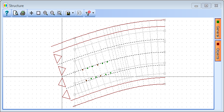
A two span grillage model of a 500mm thick, curved slab, as shown below and as defined in example 6.4 is to be loaded and analyzed for dead, superimposed dead and Eurocode traffic loading.

Layout

It is required to determine the design sagging (positive) moment at the centre of span 1 for ULS/STR combination for persistent design situations and maximum deflection along the lower edge of the structure for SLS frequent combinations of load. Engineering judgement is to be used to create just two load patterns to achieve this.

Details of the characteristic loading are as follows:

Dead load of the concrete slab is 25kN/m³ (γG = 1.35 & 1.0)
Carriageway surfacing is 0.2m thick and has a density of 18kN/m³ (γG = 1.2 & 1.0)
Footway makeup & finish is 0.35m thick and has a density of 20kN/m³ (γQ = 1.2 & 1.0)
Live traffic load gr5 (γQ = 1.35 & 1.0)

Procedure

Start the program and use the Home Open button to open the file “My EU Example 6_4.sst” created in example 6.4. Close the Project Overview with the “Done” button.
Change the sub title of the example to “Example 7.3” using the File | Titles menu option, Change the Job Number: to “7.3” and put your initials in the Calculations by: field before closing the form in the normal way.

Basic Loads

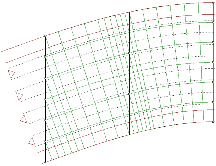
The dead load of the slab can be created by applying a volume load of 25kN/m3 to just the longitudinal members (applying it to the transverse members as well would double the actual dead load).

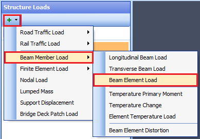
Change the navigation pane on the left hand side of the screen to Structure Loads by selecting the button at the bottom.
Click on the + button at the top to display the selection list as shown and pick Beam Member Load | Beam Element Load.
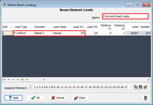
In the Define Beam Loading form, insert a new row using the table + button, then change the Load Type to “F Uniform”, the Direction to “Global Z”, the Load Value to “Volume” and Load W1 to “-25”. The field Load W2 automatically becomes “-25” also as it is a uniform load (note the units). The Name: field can be changed to “Concrete Dead Loads”.
To apply this to just the longitudinal beams we need to filter the graphics window to display just these beams. Click on the small arrow next to the filter icon in the graphics toolbar and pick Longitudinal Beams from the list.
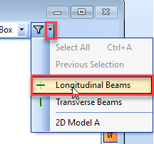
By windowing around the complete structure and changing the viewing directions to isometric it can be seen that the load has been applied to the longitudinal beams only.
Close the Beam Element Loading form with the ✓ OK button.
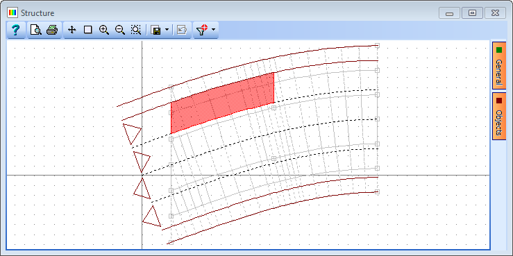
To define the Carriageway surfacing load, the Bridge Deck Patch Load option is selected after clicking on the + button at the top of the navigation window.
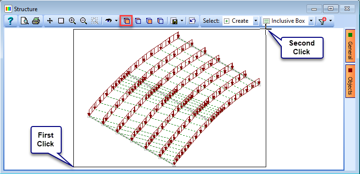
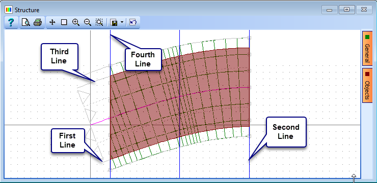
Set Define loading by: to “4 objects” then in the graphics screen click on the 4 lines bounding the carriageway area (consecutive lines must intersect). The lines are the carriageway definition lines and the construction lines at either end. It is best to click on these lines outside the bounds of the structure so as to isolate them from other lines. The loaded area is then shown hatched. (Ensure that the Carriageways box is ticked on the orange “Objects” button at the right side of the graphics screen).
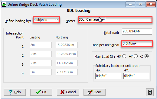
In the Define Bridge Deck Patch Loading form set Load per unit area to “3.6kN/m²” and set the Name: to “SDL: Carriageway” before closing the form with the ✓ OK button. (Note that subsidiary loads can be defined in the directions other than the main direction on the Bridge Deck Patch Load form. However, in this example only loads in the main Z direction will be defined).
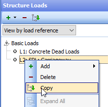
In the navigation window select the SDL load just created and right mouse click to display a context menu. Select Copy from the drop down list.
Set Define loading by: to “4 objects” (and click “Yes” on the confirm form that appears), then in the graphics screen click on the 4 lines bounding the south most footway area. (You can zoom in to click on the bottom edge of the carriageway to ensure that you do not select a beam element instead).
In the Define Bridge Deck Patch Loading form set Load per unit area to “7kN/m²” and set the Name: to “SDL: footway 1” before closing the form with the ✓ OK button.
Repeat steps 12 to 14 but for the north most footway using the Name: “SDL: footway 2”
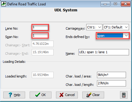
Click on the + button in the navigation window and select Road Traffic Load | LM1 UDL System to open a Define Road Traffic Load form. Set Ends defined by: to “span” and the Lane No: and Span No: to “1”. The load intensity is calculated automatically, based upon lane 1 factors (lane numbers and factors are defined at the compilation stage). All other data can be left as the default so close the form with the ✓ OK button.
Right mouse click on the UDL load in the navigation window and select Copy from the drop down list. Change the lane to “2” and close the form with the ✓ OK button.
Repeat step 17 for lanes 3 and 4.
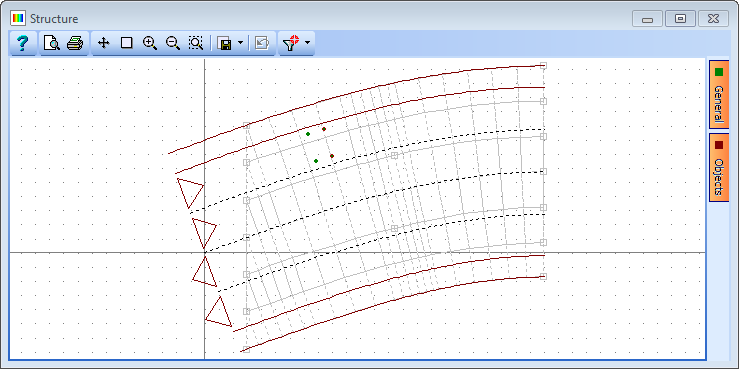
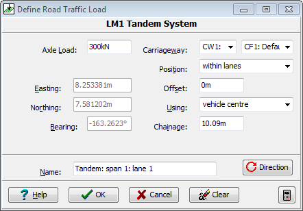
Click on + the button in the navigation window and select Road Traffic Load | LM1 Tandem System to open a Define Road Traffic Load form. Set Position: to “within lanes”, Using: to “vehicle centre”, Offset: to “0” and then position the Tandem System load approximately by clicking twice in the north most lane somewhere near the centre of span 1 (leave a gap of a few seconds between clicks). Now set the Chainage in the form to “10.09m” to position it more accurately. Close the form with the ✓ OK button.
Repeat this for lanes 2, 3 and 4 with chainages of “9.20m”, “8.25m” and “7.25”. Note that no footway live loading is applied because this is eventually going to be a Gr5 load combination.
Click on the + button of the navigation window to add Road Traffic Load | LM3 UK Special Vehicle.
Set the Model: to “SV80”, Bogie Spacing: to “1.2m” and Position: to “within lanes”. Click twice anywhere in lane 3 on the graphics screen to approximately position the vehicle. (Ensuring that you leave a gap of at least 1 second between clicks).
Set the Offset field to “0m” so that the vehicle is within the boundaries of lane 3.
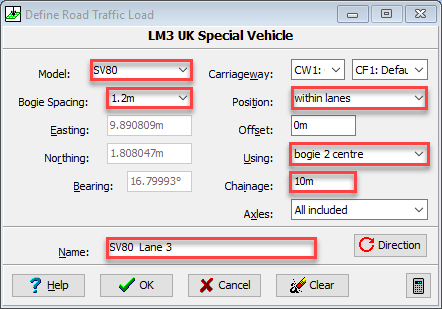
To position the vehicle longitudinally set Using: to “bogie 2 centre” and Chainage: to “10m”. Change the Name: field to “SV80 Lane 3” before closing the form with the ✓ OK button.
Repeat 21 to 24 above but place the vehicle in lane 4 and set the chainage at “9m”. Change the Name: to “SV80 Lane 4” before closing the form with the ✓ OK button.

Loading Sets

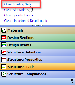
It is sometimes convenient to group the basic loads into recognisable sets. This can be done by clicking on the Open Loading Sets... option at the bottom of the navigation window.
In the Define Loading Sets form click on the + button at the top right and then change the Set Name to “Dead Loads”.
Click on the single dead load in the Unassigned Load Cases: list and then click on the “>” button to move it into the Selected Load Cases: list.
Repeat 27 and 28 above with Set Name of “SDL” and the appropriate load cases.
Repeat 28 and 29 above with Set Name of “Live Loads” and the remaining load cases. (Note that multiple loads can be selected at once by holding the shift key down while clicking on the first and last in a series) but the “>>” button also works.
Close the Define Loading Sets form with the ✓ OK button.

Compilations

Change the Navigation view to Structure Compilations by clicking the appropriate button at the bottom of the navigation window.
Click on the + button to add a Dead Loads at Stage 1 compilation. Click on the + button near the bottom of the form to add a row to the table. In this row of the compilation table use the drop down list to select the “Concrete Dead Loads” case. Select “ULS STR/GEO” from the Limit State: dropdown and click “Yes” on the confirm form. Ensure the gamma is set to 1.35. Change the Name: to “DL ULS”. Close the form with the ✓ OK button.
Repeat 33 above but this time set the Limit State: field to SLS Frequent (a prompt to confirm changing the load factors will appear) and the Name: to “DL SLS”. Note that the default gamma is correctly set at 1.0 automatically.
Click on the + button to add a Superimposed Dead Loads compilation. Click on the + button near the bottom of the form 3 times to add 3 rows to the table. In the compilation table use the drop down list to select the three SDL load cases. Select “ULS STR/GEO” from the Limit State: dropdown and click “Yes” on the confirm form. Note that the default gamma is correctly set at 1.2 automatically. Change the Name to “SDL ULS” and close the form with the ✓ OK button.
The compilation for SDL SLS can be created by copying the ULS compilation and changing the Limit State: field to “SLS frequent”. The factors are changed by the program to 1.0. Change the Name to “SDL SLS” and close the form with the ✓ OK button.
Click on the Navigation window button to add a Road Traffic Groups | GR5 compilation. Click on the + button near the bottom of the form 7 times to add 7 rows to the table. This compilation will be for ULS max sagging so select the vehicle loads as shown below.
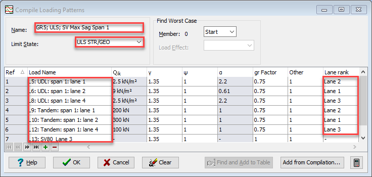
Select “ULS STR/GEO” from the Limit State dropdown and click “Yes” on the Confirm form to change the gamma factors to the correct value of 1.35. Note that the Lane rank numbers need changing as shown to correctly represent the lane factors. The Name: of the compilation should be changed to “GR5; ULS; SV Max Sag Span 1” before closing the form with the ✓ OK button.
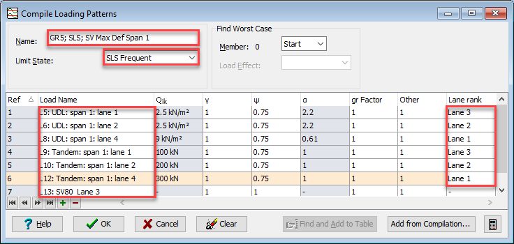
For the SLS Max Deflection Compilation repeat 37 and 38 but change the Limit State: to “SLS Frequent” and include the vehicles and Lane Rank numbers as shown below. The Name: is set to “GR5; SLS; SV Max Def Span 1” before closing the form with the ✓ OK button.

Analysis

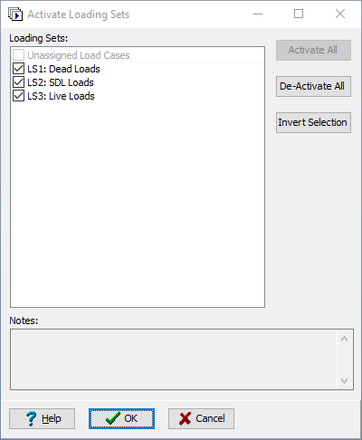
The load cases can now be solved using the main menu Item Calculate | Analyse Structure, which carries out the solution and stores results ready for viewing. Because we have defined loading sets an Activate Loading Sets form is displayed allowing a choice of which loading sets to analyse. Ensure they are all ticked and then click on the ✓ OK button.
Once the analysis is complete as indicated on the Analysis form click on the small icon at the bottom right of this form.
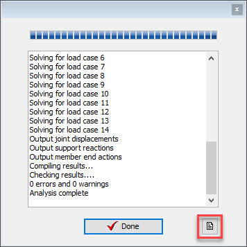
This will display the analysis log file which will indicate any warning messages about the analysis (if any) and give a summary of the analysis degrees of freedom and the total applied loads and total reactions for each load case. These should be inspected for consistency.
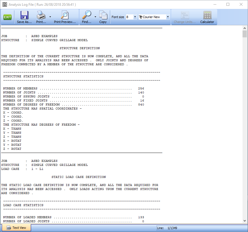
The analysis log file can then be closed using the EXIT button on the top left of the window. The Analysis form can also be closed using the ✓ Done button.

Results

The maximum sagging moments can be obtained by looking at the results of the appropriate live load compilation in the results viewer. This is opened using the menu item File | Results.
If the graphics and tabular results are not shown on the same screen then ensure that the Graphics is enabled using the menu item View | Set Default Layout | Graphic Above Table.
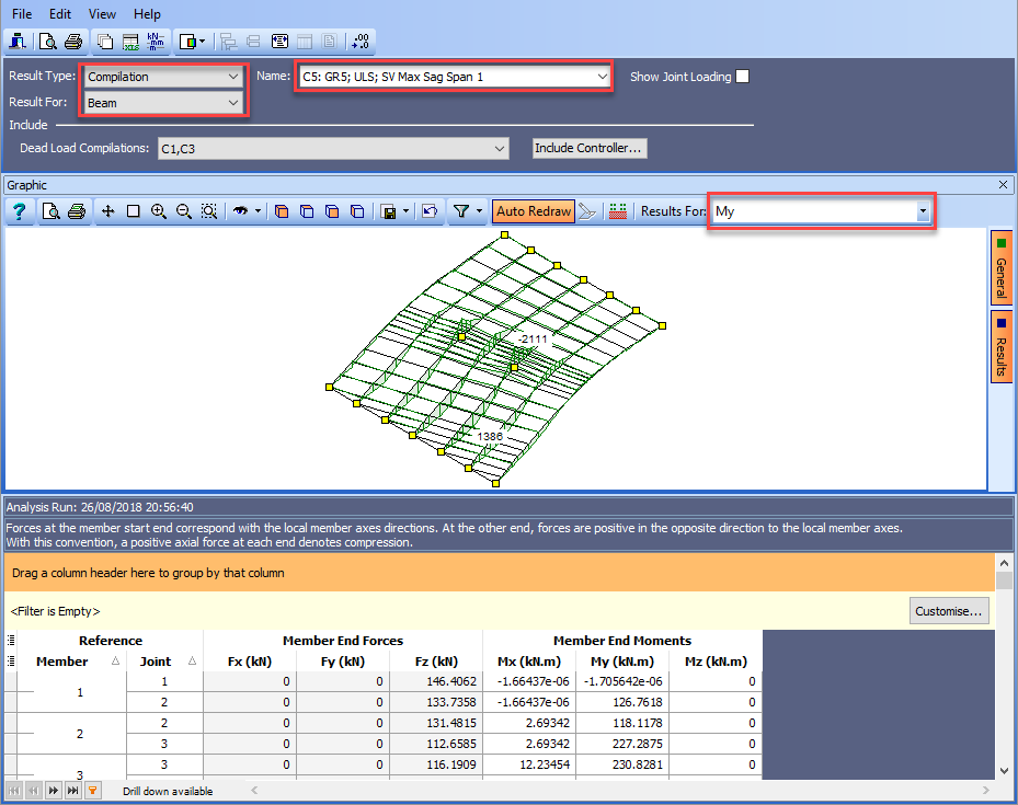
Set the Results Type: to “Compilation” and the Results For: to “Beam” and the Name of the compilation to “Gr5; ULS UDL; SV Max Sag Span 1”.
To add the effect of dead load and superimposed dead load to the live compilation results then use the drop down list in the Dead Load Compilations: field to include both ULS Dead & SDL compilations. Click on the isometric view icon on the graphics toolbar and select “My” in the Results for: dropdown menu.
To determine the maximum value then annotate the graphics using the General button at the right of the graphics screen and tick the Result tick box. If all results are shown then the “Format” button can be used to select “maximums only”. Click on the Auto Redraw button on the graphics toolbar to show the results. It is worth noting that un-ticking the “Transparent” box in the Text Setup form can make it easier to read the results in the graphics window.
To see how the graphics and table would be printed out, use the File | Print Preview menu item to display the print preview. This can be printed if required. Close the print preview using the Close toolbar button.
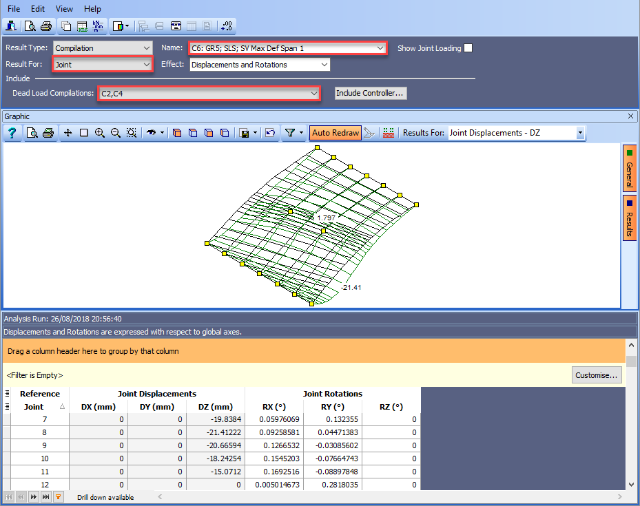
To repeat this exercise for the SLS displacements change the compilation Name to “Gr5; SLS UDL; SV Max Def Span 1”, the Results For: to “Joint” and include the SLS Dead Load Compilations, C2 and C4, in the same way as before.
To ensure that you are looking at z displacements click on any number in the DZ column in the table.
Before printing a Print Preview of these results remove columns from the table that are all zeros (DX, DY, RZ). This is done by right mouse clicking on each column header and selecting “Remove This Column” from the drop down menu displayed. These can be reinstated if required by clicking on the column control icon at the far left of the column headers and ticking the appropriate boxes.
To determine which node number gives the min result we can sort the results in ascending order for a particular column and then look at the result at the top of the table. For the vertical displacements, this is done by left clicking on the DZ column header until the sort arrow points upwards and then scrolling to the top of the table.
Close the results viewer using the File | Close Tabular Results menu item.
Save the data file, using the menu File | Save As to a file called “My EU Example 7_3.sst”
Close the program.

Summary

This example provides a basic introduction to the basic loading and results of a bridge deck grillage analysis.

Although maximum results are normally obtained using the load optimization features in Autodesk Structural Bridge Design, to position vehicle patterns accurately, it is important for the engineer to be able to create loading patterns manually based on engineering experience. By understanding this process, the engineer will be confident in checking the results produced automatically by the load optimization, which is described in Section 10 of this tutorial.

Some key features of this example are:

The copying of data items to create additional data items and then modifying them (such as loads).
Understanding Vehicle loading.
Creating load compilations for different limit states.
Grouping of loads to form loading sets. These should not be confused with compilations, as the loads or effects are not summed but merely grouped for convenience. Each group can be analyzed separately and will not require re-analysis if other groups are subsequently solved (as long as other data hasn't changed.
The production of an analysis log file (the last log file produced is always available from the File | Analysis Log File menu). This file easily gives the ability to check that the total applied loads are equal and opposite to the resultant total support reactions. It is important to do this at least once for every structural model, as differences in these values are an indication of an ill-conditioned stiffness matrix and that structure stiffness should be scrutinized.
To show the ability to customize and be selective on printed output.