
2D conduits can be used in a 2D simulation to introduce unidimensional hydraulic structures directly in the 2D engine, and allow flow to be transferred between two areas of a 2D zone in an InfoWorks network. 2D conduits also provide a way of introducing a linear object to capture surface flow directly from the 2D mesh to transfer it into the drainage system, providing an alternative to the current method of using point objects such as manholes of flood type 2D.
A conduit is defined as a 2D conduit if its type is:
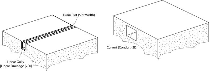
- Conduit (2D) - which represents a drainage structure such as a culvert, which, for example, may be located beneath a road.
This type of 2D conduit is modelled directly in the 2D engine, which avoids the need to use a 1D network with 2D manholes/inlet/outfall nodes (which does not consider transfer of momentum) or modifying the ground model to accommodate the drainage structure using a Base Linear Structure (2D). In addition, momentum is preserved in the 2D conduit/2D zone connection, providing a better representation of the actual flow for this type of hydraulic structure.
Tip: Alternatively, a Culvert (2D) type of conduit can be used for 2D modelling of a culvert. This uses empirical flow equations rather than the shallow water equations (see Flow calculations below) that are used by a Conduit (2D). - Linear Drainage (2D) - which represents a linear gully, such as a slot drain, which is connected vertically to the 2D surface.
This type of 1D-2D linear connection can be used where the drain slot or trench is much longer than the equivalent face length of the default 2D element area defined on 2D zones. For example, the default 2D element area defined on 2D zones is 100m2 thus the equivalent face length is 15m for a triangular 2D element. Therefore, this type of conduit could be used where a drain slot is much longer, for example 50 to 100m, than the face length. Such types of drainage systems are used on roads and large infrastructures, such as airports. A typical modelling scenario which may use this functionality would be detailed drainage site projects, where the 2D modelling resolution is in the order of 100m2 or less.
A 2D conduit can be connected to a 1D node, but it will only be included in a 2D simulation if it is connected to a Connect 2D type of node within the 2D zone. There are 4 types of connection for Connect 2D nodes - Break, 2D, Open and Lost - each of which defines the way a 2D conduit exchanges flow at the upstream/downstream end vertex. See the section Edge linkage for further information.
The following figure illustrates how the flow may be represented on the GeoPlan and in the 3D View when replaying the results of a simulation that includes a Linear Drainage (2D) type of conduit.
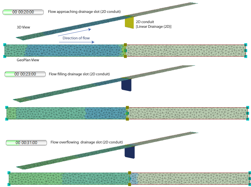
The storage capacity of the Linear Drainage (2D) conduit is included in the flow calculations which are described in the following sections.
Flow calculations
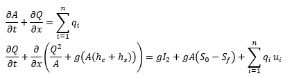
Flow in the 2D conduits is represented by the one dimensional version of the Shallow Water Equations (SWE) whose conservative formulation for the mass and momentum equations can be expressed as shown below:
|
|
where: A is the wet area (m2) Q is flow (m3/s) qi is the net source discharge per length (m/s) ui is the velocity of the ith net source discharge (m/s) hc is the distance between the free surface and the centroid of the flow cross-sectional area (m) hs is the pressure head under pressurized flow conditions (m) I2 is the pressure forces due to conduit changes in width (m3) g is the gravity acceleration (m2/s) S0 is the bed slope Sf is the bed friction n is the number of source discharges |
2D conduits are subdivided into a series of computational cells. Computational cells in Conduit (2D) conduits are generated using the existing procedure for standard conduits. An additional check prevents a computational cell from being smaller than the specified Min Space Step.
For Linear Drainage (2D) conduits, the computational cell discretization depends on the database version. For databases earlier than version 2027.1, a computational cell is generated for each 2D mesh face followed by the conduit. For databases at version 2027.1 or later, contiguous 2D mesh faces connected to the same 2D element are grouped into a single computational cell. This can reduce timestep restrictions caused by very small internal cells, particularly in models that use clip meshes.
The one dimensional SWE are discretized on each computational cell using a first order explicit scheme and solved following an analogous numerical scheme to the one deployed in the 2D engine; a finite volume formulation based on the Godunov scheme with the numerical fluxes calculated using the standard one dimensional Roe’s approximate Riemann solver.
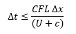
The time step in the 2D conduits is calculated using the standard Courant-Friedrichs-Lewy condition which has to be fulfilled at the computational cells. The minimum between the time step calculated in the 2D conduits and the 2D time step is used as the global time step by the 2D engine.
Courant-Friedrich-Lewy condition is:
|
|
where: CFL is the dimensionless Courant number (the Timestep Stability Control set in the 2D parameters. Default=0.95) u is velocity (m/s) c is the flow celerity calculated as √g A/W (m/s) Δt is the time step (s) Δx is the computational cell length (m) |
Edge linkage
Flow calculation, when a 2D conduit is connected to a Connect 2D type of node, depends on the type of connection:
- Closed - no flow through the edge. Used, for example, at the upstream edge of the 2D conduit.
- Lost - any flow through the edge is lost. The 2D engine assumes uniform flow conditions at the edge.
- 2D - indicates that there is a connection to an element in the 2D surface. The hydraulic variables in the 2D element are used as a boundary condition in the 2D conduit. For subgrid 2D elements, these hydraulic variables are calculated at the 2D triangle where the Connect 2D node is located. The flow exchange between the 2D element and the 2D conduit includes momentum.
- Break - used to connect two 2D conduits. Flow is calculated as if the two 2D conduits are joined together and that the break type of Connect 2D node does not have any storage. Momentum is preserved.
- 2D line - indicates that there is a connection to multiple elements in the 2D surface. For subgrid 2D elements, hydraulic variables are calculated at the 2D triangles intersected by the 2D line connect. The specified 2D line connect object represents the flow exchange boundary.
A 2D conduit can also be connected to a 1D node. If this is the case, the level at the node is set as a boundary condition for the 2D conduit and is assumed constant for the minor 2D timesteps between two major 1D timesteps. The resulting accumulated flow through the edge is added to the 1D node as an inflow in the next major timestep.
Boundary conditions at Connect 2D nodes
When an inflow (qin) or level (lev) boundary is attached to a Connect 2D node, the boundary is applied according to the connection type. Inflow is supported for Closed and Lost connection types; level boundaries are supported for Lost connection types. If both inflow and level are defined for a Lost connection type, the level takes precedence. The inflow to the Closed connection type doesn't conserve momentum, but an inflow to the Lost connection type does. For other connection types, inappropriate boundaries are ignored and a warning is issued.
Slot linkage
Linear Drainage (2D) conduits are connected to a 2D Zone and included in the mesh. The conduit is connected to the 2D surface through a slot, which acts as additional storage.
For databases earlier than version 2027.1, each computational cell corresponds to a 2D mesh face and has a vertical connection to the 2D surface. For databases at version 2027.1 or later, contiguous 2D mesh faces connected to the same 2D element are grouped into a single computational cell. Each cell has a vertical connection, and each vertical connection can contain multiple segments. Each segment corresponds to a 2D mesh face.
The calculation of the flow exchange between the Linear Drainage (2D) conduit and the 2D surface will only begin when the connected 2D element is wet, ie, the depth exceeds the Depth threshold set in the 2D Parameters dialog. The flow exchange is calculated for each computational cell as follows:
- If the capacity of the Linear Drainage (2D) conduit is exceeded, the excess of flow is poured into the connected 2D element.
- If the capacity of the Linear Drainage (2D) conduit is not exceeded and there is depth in the connected 2D element, then there will be flow into the 2D conduit. If there is still capacity on the main conduit of the computational cell, the flow will be calculated based on a standard orifice equation (see Equations 1 and 2 in the Orifice Controls topic, where the discharge coefficient is set in the Vertical connection coefficient field in the conduit properties), driven by the 2D element depth. If the only capacity available in the 2D conduit is in the slot, then the slot will be filled up instantaneously with as much water as it is available in the connected 2D element.
Pressurisation
Pressurisation at 2D conduits is supported by means of the standard Preissmann slot approach. In the case of 2D conduits of the type Linear Drainage 2D, the slot is not conceptual but real and set by the user in the Slot width conduit parameter. In the case of 2D conduits of type Conduit (2D) the slot assumptions are analogous to those used in standard conduits.
Results
The results of a simulation that includes 2D conduits and Connect 2D nodes can be displayed on the results grids for links and nodes, or on the applicable property sheet while viewing a replay of a simulation.
Meshing
The conduit type determines whether or not the geometry of the object will act as a break line in the meshing. Linear Drainage (2D) conduits act as a break line for triangulation during meshing but Conduit (2D) ones do not and are therefore not included in the 2D mesh.
For models containing Linear Drainage (2D) conduits that are updated to version 2027.1 or later, remeshing is recommended to make full use of the updated discretization.