6.5 Finite Element Slab

Subjects Covered

• Refined Analysis
• 2D
• Transition Curve Design Lines
• Construction Lines
• Meshing
• Slab Properties
• Support Conditions
• Data Reports

Outline

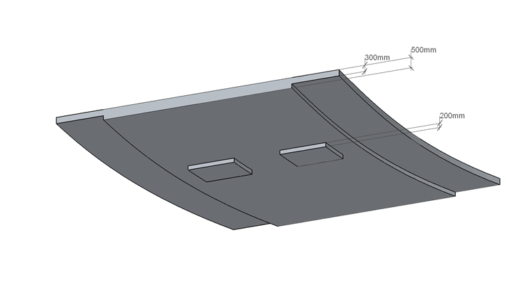
A concrete slab is shown below which has the same setting out dimensions as the slab in example 6.4. It is to be modelled as shell finite elements in Autodesk Structural Bridge Design and the data file saved for analysis in Section 7.

The slab is generally 500mm thick but has a 2.5m wide cantilever on either edge which is 300mm thick.

It is supported on 5 discrete bearings at each end of the slab and 2 bearings at midspan. The layout and restraint conditions of the bearings are the same as for example 6.4 except the four corner bearings are excluded.

Around the location of the two midspan bearings, the slab is thickened to 700mm so as to form a column head. The lateral dimensions of this thickened slab are defined by the mesh layout.

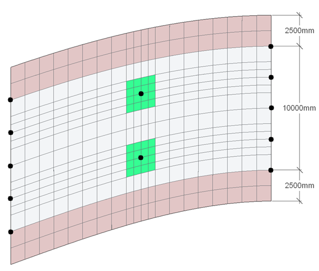
The mesh Layout is shown below where both longitudinally and transversely, the wider elements are twice the width of the narrower ones.

The single Carriageway is 12m wide with a 1.5m verge on either side and is centred on the deck, as in example 6.4.

The concrete is grade C40/50 so it will have an elastic modulus of 35.2205GPa. Poisson's ratio is assumed to be 0.2.

Procedure

Setup

1. Start the program, close the Home using the ESC key and open the supplied data file “EU Example 6_4 Curved Slab Layout.sst” via the menu item Help | Tutorials | Open Tutorial Model. This will give us the basic setting out from which we can create the FE model.
2. Use the File | Titles menu option to set the Project Title to “Curved FE Slab Model” with a sub title of “Example 6.5”.
3. Set the Job Number to “6.5”, put your initials in the Calculations by: field and close the form with ✓ OK.

FE mesh

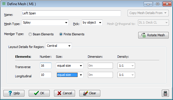
4. We can now define the two meshes. Left mouse click and then right mouse click on the 2D sub Model in the navigation window and select +Add | Mesh. This will display the Define Mesh form.

5. Set_ Name:_ to be “Left Span”, Mesh Type: to be “Splay”, Pick: “by object” and Member Type: to “Finite Elements”.

   

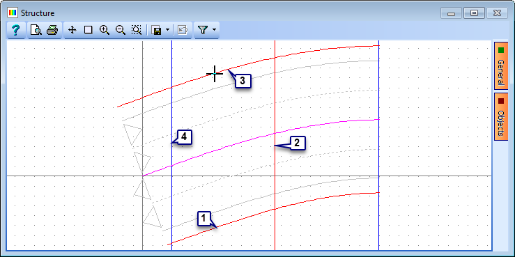
   The boundary of the mesh is then picked graphically by selecting the four boundary edges of this span. They must be picked so that consecutive lines intersect (in order) and the first line defines the general longitudinal direction, the second defines which is the positive direction (as can be shown by the arrow in the graphics).

6. Start on the bottom verge line, then the middle construction line, next the top verge line and lastly the leftmost construction line.

   

7. Set the no. of Tranverse no of elements to “16” and Longitudinal to “10” and note the change in the graphics.

8. The spacing of the elements now needs to be adjusted so that the four elements either side of each of the central supports is half the size of the others. Change the size field for the transverse spacing from “equal size” to “set size”.

9. This opens the Set Transverse Size form. The spacing factors can be set to “0.5” where narrow elements are required as shown below:

   

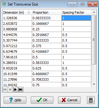
10. The other values of Dimension and Proportion are updated automatically. (the form above does not show the full table and there are three spacing factor values of 1 that are not shown). Close this form with the ✓ OK button.

11. Set size is used again, for the longitudinal spacing, but it is only the last two rows in the table that have the spacing factors changed to “0.5”.

12. Close the Define Mesh form with the ✓ OK button.

13. Repeat 20, 4, 5 and 6 for the second mesh but set the Name to “Right Span” and pick the boundary of the right span.

14. The general mesh parameters, such as spacing, can be copied from the first mesh by clicking on the “Copy Mesh Details From” button and selecting that mesh.

15. The longitudinal spacing will need adjusting for this mesh to set the narrower elements at the start. To do this re-select “set size” for the Longitudinal spacing and then set the Spacing Factors such that they are all 1, except the first two, which will be “0.5”. Close this form with the ✓ OK button.

16. Close the Define Mesh form with the ✓ OK button.

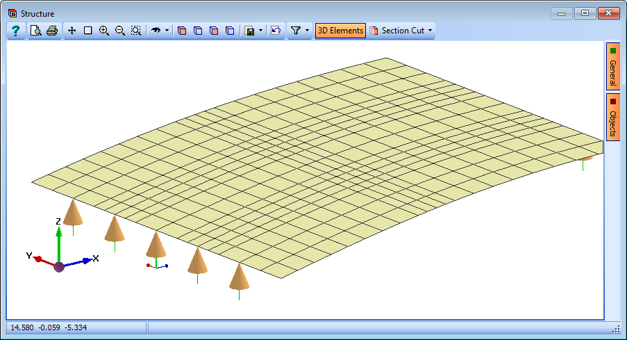
17. Click on the Refined Model node in the navigation window and in the graphics screen change the viewing direction to plan view by using the 3D view icon . The mesh should now look like the picture below:

    

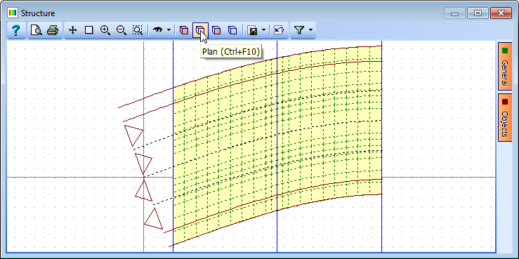
Span End Lines

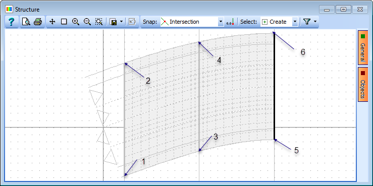
18. Before positioning supports we will define the span ends by drawing the span end lines. This is done by right clicking on Structure in the navigation window and selecting +Add | Span End Lines.

19. The coordinates of each end of the lines could be entered manually into the table but it is easier to set the Snap: mode (Graphics toolbar) to Intersection and pick the joints of the mesh coinciding with the span ends. The sequence of clicks to give three lines would be as follows:

    

    

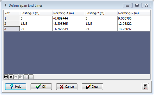
20. Close the Define Span End Lines data form with the ✓ OK button.

Supports

21. Click the button at the top of the navigation window and select Supported Nodes to open the Define Supported nodes form.

    Five nodes along the two outer span end lines and two of the nodes along the middle span end line need supporting.

22. In the graphics window toolbar set the second Select: option to “All Joints” and then click on the required supported joints as shown below.

    

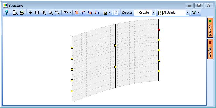
23. In the Define Supports table you will see that the Group Type: is set to Uniform, which means all the support conditions are the same. Set the restraints such that all degrees of freedom are Free except Direct Restraint Z, which is Fixed.

24. Now change the Group type: to Variable, which allows each support to have different constraints applied.

25. To fix the X and Y translational constraints on the centre support along the left span end line we first click on it in the graphics screen (which highlights it in the table). In this row of the table we change the X and Y Direct Restraints to Fixed.

26. Item 24 is repeated for the centre support under the right span end line except that we only change the Y Direct Constraint to Fixed.

    

27. Close the Define Supported Nodes form using the ✓ OK button.

28. To graphically see the support directions and type it is required to open a 3D elements view. This is done using the File | 3D Elements View... menu item.

    

    All the supports will be visible if “Wire Frame View” is selected from the side form when clicking on the General button. Remember to switch this off before closing the 3D Elements View, by double clicking on the Structure item in the Navigation window, as this affects all graphics windows.

Properties

There are three properties to define:

• The 700mm thick isotropic FE property.
• The 300mm thick isotropic FE property.
• The 500mm thick isotropic FE property.

29. We first change the navigation window to Structure Properties.

30. Click on the button at the top of the navigation window and select Finite Element.

31. In the Finite Element Properties form, change the Thickness: to “700” and selecting the Material Property: to be “MP2: C40/50”.

    

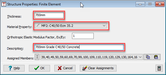
32. Change the Description: to “700mm Grade C40/50 Concrete”.

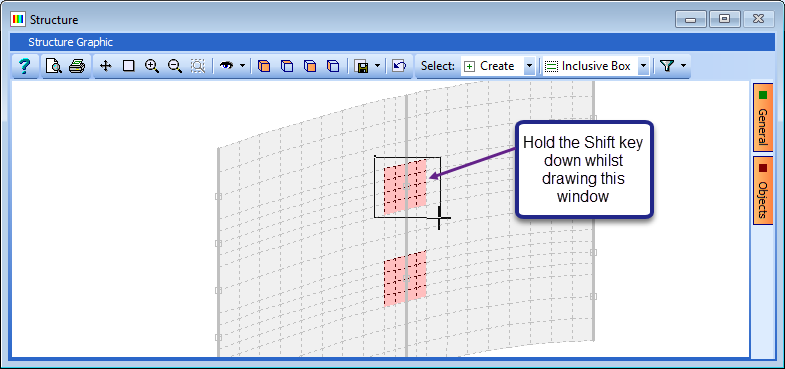
33. Select the 32 elements in the graphics window surrounding the two central supports as shown. This can be done by clicking on the individual elements or windowing around the two groups. To create the window, the “Shift” key on the keyboard must be held down whilst clicking the two opposing corners. Ensure that Select: is set to “Inclusive Box” in the graphics window.

    

34. Close the Finite Element Properties form with the ✓ OK button.

35. Right mouse click in the navigation window on the property just defined and select “Copy."

    

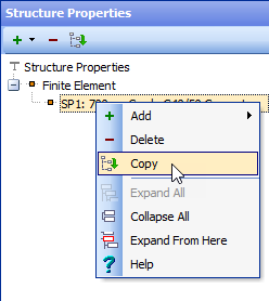
36. Set the Thickness: to “300”, the Description: to “300mm Grade C40/50 Concrete” and then select the two rows of element adjacent to each curved edge of the slab.

37. These elements can be selected by clicking on them individually, windowing around them in groups or, if we know the element numbers, they can be listed as a text sequence eg. “25 to 50”.

    

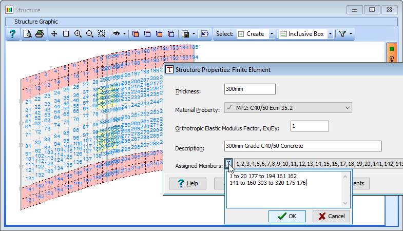
38. To determine the element numbers they can be annotated on the graphics by clicking on the orange “General” button on the right of the graphics screen and then ticking the tick box (if this is not shown click on the button “Switch to Member No.”). Zooming in and panning should show the numbers to be:

    • 141 to 160 1 to 20
    • 303 to 320 177 to 194
    • 161 162
    • 175 176

39. To enter this text sequence click on the small text icon at the left end of the Assigned Members: field and type in the text as shown into the text field displayed (remembering to click ✓ OK on the sub-form).

40. Turn off the Element Annotation in the graphics window.

41. Close the Finite Element Properties form with the ✓ OK button.

42. Right mouse click in the navigation window on the property just defined and select “Copy”.

43. Set the Thickness: to “500”, the Description: to “500mm Grade C40/50 Concrete” and then select the remaining elements of the slab in the graphics window.

44. This can be done by windowing around the whole structure and then answer No to all when asked if you wish to overwrite previous assignments

45. Close the Finite Element Properties form with the ✓ OK button.

46. Save the data file using the main menu File | Save as with a name of “My EU Example 6_5.sst”.

Data Reports

For general data reports and graphical plots follow the procedures detailed in previous examples (in particular example 6.4).

It is required to produce a report for the section properties of a specific finite element to show items such as element area and aspect ratios.

47. In the main menu select File | Data Reports.

48. In the Data Reports form, select the Member Section Properties tab and ensure that only Show Summary is ticked.

    

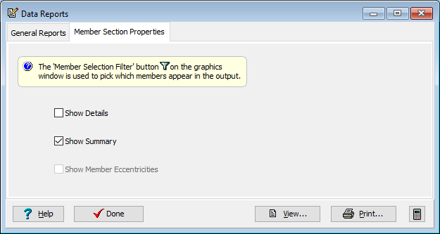
49. In the graphics window toolbar, click on the Filter icon to open the Member Selection Filter form and click on the bottom left hand element in the display before closing the form with the ✓ OK button.

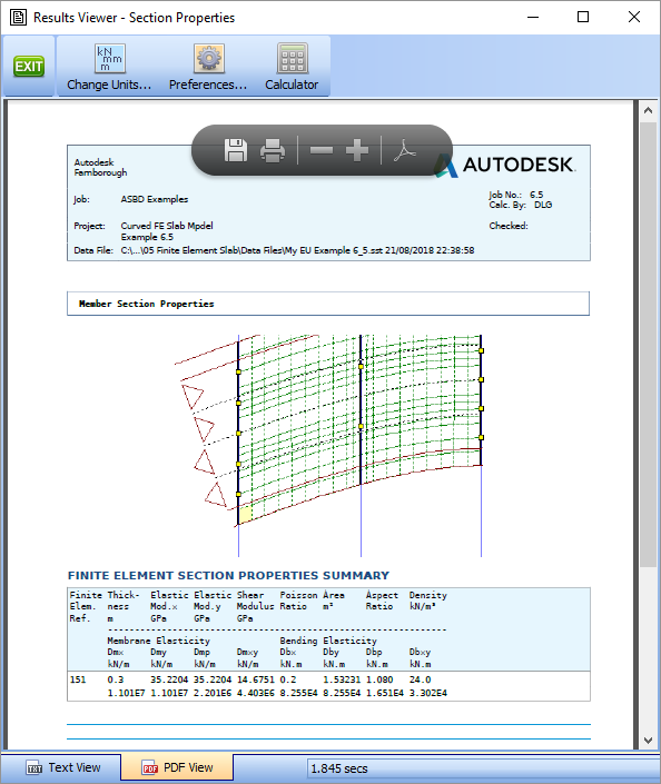
50. Click on the View... button on the Data Reports form to show the basic Results Viewer. Although this doesn't show the graphics directly, if this form is printed (or print preview) it will have the current graphics included at the top of the report.

51. Alternatively, if it was required to save a PDF file of this report then click on the “PDF View” tab at the bottom of the Data Reports form. This view can be saved as a local PDF file.

    

52. Close the Results Viewer using the green Exit button and then close the Data Reports form using the ✓ Done button.

53. Close the program.

Summary

This simple FE mesh of a curved flat slab highlights all the basic methods for creating any FE mesh structure and introduces most of the tools required to create an FE mesh and get data reports. The model that has been saved will be used in the loading and analysis of this structure in Section 7 of this tutorial.