Guidelines for using Remove rigid body modes
Remove rigid body modes can be used when either of the following conditions are true:
The model is fully unconstrained
That is, you have not applied any X, Y, or Z constraints to any portion of the model. When the model is fully unconstrained, applied loads can be balanced or unbalanced.
The model is constrained,
- AND all loads acting in the constrained direction are balanced
- AND the sum of the moments equal zero.
- the loads are NOT balanced, when you activate Remove rigid body modes, the loads that are added to balance the loads and moments essentially change the reaction forces, and the results are wrong.
- the loads and moments ARE balanced, when you activate Remove rigid body modes, no additional loads are applied and the reaction forces and results are correct.
Table 1: When to activate Remove rigid body modes.
| Is the model constrained? | Are forces balanced in the constrained directions? | Does the sum of the moments = 0? | Can you use Remove rigid body modes? |
|---|---|---|---|
| No | -- | -- | Yes |
| Yes | Yes | Yes | Yes |
| Yes | Yes | No | No |
| Yes | No | No | No |
Constrained model
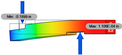
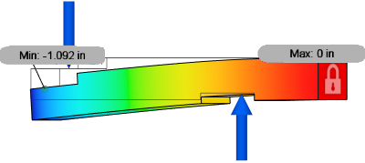
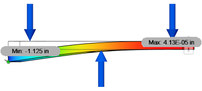
Example 1: Loads are balanced but the sum of the moments does NOT equal zero
Assume that a model is constrained against movement in the vertical direction. A force of 100 N is applied in that direction. The model must have an opposing force of 100 N in the opposite direction so that the sum of forces in the vertical direction is zero. Loads acting in unconstrained directions may be balanced or unbalanced.
 |
 |
| Remove rigid body mode not enabled, showing correct deflection | Remove rigid body mode enabled, showing incorrect deflection |
Because the moments due to the forces do not equal 0, the results are wrong when Remove rigid body mode is enabled. Notice that the reaction moment is zero, due to the solver adding a rotional acceleration to counteract the unbalanced moment.
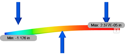
Example 2: Loads are balanced AND the sum of the moments equals zero
Assume that a model is constrained against movement in the vertical direction, with a force of 100 N applied in opposing directions. (One force of 100 N pointing up, and two forces of 50 N each pointing down.) Because of the equal spacing in this example, the moment due to the three loads equals zero. The remove rigid body modes option can be used in this example if necessary.
 |
 |
| Remove rigid body mode not enabled, showing correct deflection. | Remove rigid body mode enabled, showing correct deflection |
Unconstrained model
When using Remove rigid body mode with an unconstrained model, it is still important to consider whether you must balance the applied loads to achieve accurate results. Examples 3 and 4 demonstrate two situations. One scenario produces good results with an unbalanced load. For the other scenario, you need to balance the loads to achieve accurate results.
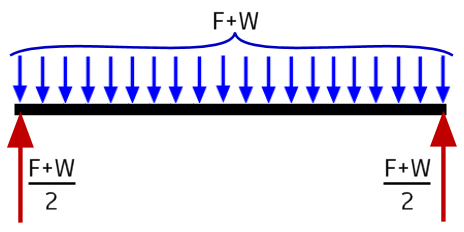
Example 3: Unconstrained - Unbalanced applied loads are acceptable
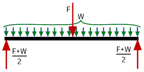
This example is a simply-supported square bar with a uniformly distributed force (F) applied to the full length of the bar. The reaction at each end is (F + W) / 2, where W is the weight of the bar itself. You can apply only the reaction forces to the ends of the bar (red arrows). The acceleration applied by the solver produces a force (Fa) equal to F + W (blue arrows). A portion of this acceleration force acts on every element in the model. The resultant counterforce to the applied load is distributed uniformly along the full length of the model.
Alternatively, if you perform the following two actions:
- Apply the distributed force (F) to the length of the bar
- Activate the gravity load, producing the weight load (W)
Then, the result is identical to the fully unconstrained case. The solver only has to apply a very small acceleration to counter the small mathematical imbalances resulting from the FEA method.
Example 4: Unconstrained - Balanced loads must be applied for correct results
In this example, you apply balanced loads to the model, which theoretically provide an equilibrium condition. The solver applies a very small amount of global acceleration, just enough to counter the slight mathematical imbalance introduced by the FEA method.
Apply a large force (F, the middle red arrow), concentrated at the center of the span. Activate gravity to produce the weight load (W, the green arrows). Finally, apply the calculated reaction forces to the ends of the bar (the outer two red arrows). When a load acts at a point, edge, or small area of a part, the solver cannot accurately represent it by applying global acceleration. The distributed force from global acceleration and a concentrated force at midspan do not produce the same stress or displacement results.