Set up Events
There are four parameters that define the event duration and time step size in a transient heat transfer analysis. These are specified in the Event section of the Analysis Parameters dialog. The analysis can be split into multiple time intervals, and each interval can use a different time step size. For example, immersing a hot piece of steel into a liquid bath results in rapid cooling at the very beginning of the analysis: use small time steps in this interval. As the part stabilizes, larger time steps can be used for faster solution.
- The Initial Time input is the time at the start of the analysis. This value is usually zero but could be another value if restarting an analysis from another model, or for convenience.
- The Time column in the spreadsheet is the time when the interval ends. The Time in the first row needs to be later than the Initial Time, and the time in each row needs to be later than the previous row.
- The Steps column in the spreadsheet is the number of steps used in the time interval, where the interval runs from the time on the previous row and ends at the time on the current row. Thus, the time step size dT for row i is as follows: dT = [Time(i)Time(i-1)]/[Steps(i)]
- Although the results will be calculated for each time step, the output interval can be set to limit the amount of output. The Output Interval column specifies how many calculation steps are output. (These results are displayed in the Results environment.) A value of 1 indicates that all calculation steps are output, 2 indicates that every other step is output, and so on.
Define Load Curves
In a transient heat transfer analysis, all the loads follow load curves. The load curves are defined in the Analysis Parameters dialog by pressing the Load Curves button. Refer to the table below to determine how the value in the Factor column of the load curve will affect each thermal load parameter.
| Parameter | How Factor Affects Parameter |
|---|---|
| Applied temperature magnitude | See the page Applied Temperature |
| Convection coefficient | Multiplies |
| Convection ambient temperature | See the page Convection |
| Radiation function | Multiplies |
| Radiation ambient temperature | See the page Radiation |
| Surface heat flux | Multiplies |
| Internal heat generation | Multiplies |
| Nodal heat source | Multiplies |
| Body-to body radiation ambient temperature | Multiplies |
There are two methods that can be used to create the load curves. If you select the Piecewise Linear radio button in the Load Curve Form section, you will be able to define the load curve by defining several times and the corresponding factors. The factor values will be linearly interpolated between the defined times. If you select the Sinusoidal radio button in the Load Curve Form section, you will be able to define the parameters of the sinusoidal curve in the fields below.
Multipliers
There are four multipliers that will control the magnitudes of various thermal loads when they are applied to the model. These are located in the Multipliers tab of the Analysis Parameters dialog.
- The value in the Boundary temperature multiplier field will multiply the magnitudes of any applied temperatures on the model.
- The value in the Convection multiplier field will multiply the convection coefficients for any convection loads on the model and any surface heat fluxes. (Nodal heat fluxes are not affected by any multiplier.)
- The value in the Radiation multiplier field will multiply the radiation functions for any surface radiation loads on the model. Body to body radiation is not affected by this multiplier.
- The value in the Heat generation multiplier field will multiply the magnitudes of any internal heat generation loads on the model.
A value of zero in any of these fields except for the Boundary temperature multiplier field will disable the loads of that type in the model. A value of 0 in the Boundary temperature multiplier field will change the magnitudes of the applied temperatures to 0 degrees.
Default Nodal Temperatures
The value in the Default nodal temperatures field in the Options tab of the Analysis Parameters field will be used to define the initial temperature of any node that does not have an initial temperature defined. (Unless your transient analysis is starting at a temperature of zero, the temperature at the beginning of the analysis needs to be specified.)
The results of a previous thermal analysis can be used as the initial temperature profile for a transient heat transfer analysis. There are two methods to do this.
Method 1:
Select the appropriate analysis type in the Source of initial nodal temperatures drop-down box on the Options tab. Select the model in the Existing model field. If you are using another transient heat transfer analysis and want to use an intermediate time step, select the Specified option in the Time step from heat transfer analysis drop-down box and specify the time step in the Time step field. This capability provides the opportunity to do a restart analysis as follows. (See also Restarting an Analysis below for additional restart capabilities.)
In some cases, it may be desirable to split a transient analysis into separate analyses instead of trying to describe the entire load curve in one analysis. For example, several scenarios of cooling may need to be investigated after the part is heated. Thus, one file could be used to analyze the transient heating of the part, and then separate files could be used to analyze each cooling scenario. To accomplish this, the initial temperature for the second model (the restart analysis) is chosen as the final temperature from the first model. This is specified on the Options tab of the Analysis Parameters dialog.
The same procedure can be used repeatedly for a multi-phased transient analysis where parameters are changed from one analysis to the next. In this case, the procedure would be as follows:
- Build the model for the first transient or steady state heat transfer analysis (model1).
- Run the heat transfer analysis
- Adjust the existing model as needed for the second phase and save it under a new name (model2).
- Specify that the initial temperatures for model2 are the final temperatures from model1 using the Options tab of the Analysis Parameters dialog.
- Run the analysis for model2.
- Adjust the model as needed for the third phase and save it under a new name (model3).
- Specify that the initial temperatures for model3 are the final temperatures from model2.
- Run the analysis for model3.
- Repeat as necessary for each phase.
Method 2:
- With nothing selected, right-click in the display area of the FEA Editor. Select the Loads from File command.
- Press the browse button in the Results File column. A dialog will appear which will allow you to select the results file. Use the Files of type: pull-down to select Thermal Results File (*.to, *.tto).
- Select the file with the temperature results and click the Open button.
- Only the temperatures from a single load case or time step in the selected file can be applied to the new thermal model. Select the desired load case or time step in the Load Case from File column.
- Since these temperatures are the initial temperatures, they do not need to be assigned to any Thermal Load Case; enter a dummy value in the Thermal Load Case column.
- If you want the temperatures to be multiplied by a constant value before being applied to the model, specify the constant value in the Multiplier column.
- Press the OK button.
- The nodal coordinates in the results model must be identical to the coordinates in the new thermal model when using this method. Extra nodes in either model or coordinates that do not match are ignored.
- However, this method should not be used when more than one node exists at the same coordinate in space. This occurs most often when the contact type is something other than bonded and the parts are in contact. For example, surface contact creates two nodes (one on each part) at the same coordinate. You cannot control which temperature from the matched nodes are transferred to which node; therefore, method 1 should be used in such situations.
Calculate Liquid Fractions
When any of the parts have a phase change material model included, the calculation of the liquid fraction is chosen with the Liquid fraction relationship pull-down on the Options tab of the Analysis Parameters dialog. The options available are as follows:
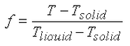
- Linear relation: The fraction of liquid f is calculated from
- Scheil relation: The fraction of liquid f is calculated from
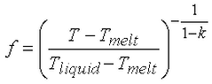
Since the equilibrium partition coefficient and melt temperature are involved, this method is generally used only with alloys.
where
- T is the calculated temperature at the node and T solid < T <T liquid .
- T solid is the solidus temperature entered in the material properties.
- T liquid is the liquidus temperature entered in the material properties.
- T melt is the melting temperature of the solvent entered in the material properties.
- k is the equilibrium partition coefficient entered in the material properties.
When the node is cooler than the solidus temperature, the fraction is equal to 0. When the node is warmer than the liquidus temperature, the fraction is equal to 1.
Import Electrostatic Results Joule Heating
If you have previously run an electrostatic current and voltage analysis on a model with identical geometry and mesh to the model that you are currently analyzing, you can apply the electrostatic results to this model to determine the temperature effects of the current. There are a few guidelines that must be followed in this process.
- You must have run an electrostatic current and voltage analysis. The electrostatic field strength and voltage analysis will not provide the necessary current information.
- The electrostatic model must be identical in geometry and mesh to the thermal model. The power generation will be applied according to part and element numbers. Therefore, it is important that the models have identical part and element numbering which is dependent on the geometry.
- You must assign a Heat generation multiplier in the Multipliers tab. This value will be used to scale the heat generation effects of the current.
- You must apply a heat generation load to the parts for which you want the Joule effects to be calculated. This number is simply a flag that allows you to control the joule effects on a part to part basis.
- Activate the Use electrostatic results to calculate Joule Effects check box in the Electrical tab of the Analysis Parameters dialog. Specify the electrostatic results file in the Source Model field.
Solver Options
Solution Options Section
The type of solver for a thermal analysis can be selected in the Type of solver drop-down box in the Solution tab of the Analysis Parameters dialog. See also Types of Solvers Available for background information. The options available are as follows:
- Automatic:. If this option is selected, the processor will choose between the Iterative (AMG) and Sparse options based on the model size. The sparse solver will be the optimum solver for mid-sized models. The iterative solver will be the optimum solver for large models and will require less RAM. If a 64 bit processor is available on the system, the iterative and BCSLIB-EXT solvers will take advantage of it.
- Sparse: Uses one of the available sparse solvers available in the Type of sparse solver drop-down box. The sparse solvers will use multiple threads/cores when available.
- Iterative (AMG): Uses an iterative scheme to solve the system of equations. The iterative solver uses multiple threads/cores when available.
- Iterative (PBiCGStab): This option is available for models containing body-to-body radiation. There are two preconditioners available for the solver in the Pre-conditioner drop-down box (see description below).
If for some reason you want to create the solution matrix but not perform the analysis, activate the check box for Stop after stiffness calculations. The only time this would be useful is to access the equation number matrix. The stiffness matrix is always calculated when running an analysis, so there is no advantage to use this option in normal circumstances.
For the sparse and iterative solvers, the Percent memory allocation field controls how much of the available RAM is used to read the element data and to assemble the matrices. A small value is recommended. (When the value is less than or equal to 100%, the available physical memory is used. When the value of this input is greater than 100%, the memory allocation uses available physical and virtual memory.)
As listed above, some of the solvers take advantage of multiple threads/cores available on the computer. The drop-down Number of threads/cores control is enabled in such situations. You want to use all the threads/cores available for the fastest solution, but might choose to use fewer threads/cores if you need some computing power to run other applications at the same time as the analysis.
Iterative Solver General Options Section
If the iterative solver is chosen, then the Iterative Solver section will be enabled. The input for this section is as follows:
- The Convergence tolerance field will determine how accurate of a solution is found to the matrix of equations. The smaller the tolerance, the more accurate the solution.
- Maximum number of iterations will stop the analysis if the matrix of equations is not solved within this number of iterations. Attention: The accuracy of the solution depends on the convergence tolerance; a smaller tolerance will result in a more accurate solution but may take more iterations. As with any iterative solution, the results should be checked to confirm that they meet the desired accuracy. In some cases, performing the analysis twice with a different convergence tolerance is the best way to confirm the accuracy.
PBiCGStab Options Section:
If the Iterative (PBiCGStab) solver is chosen, then the following input will be enabled:
- The Pre-conditioner drop-down is used to select the method used for the initial guess for the solution of the matrix when the Iterative PBiCGStab solver is chosen. The ILU(0) option is the faster and more efficient option. However, the SSOR option will require less memory. For large models, it may be necessary to use the SSOR option.
- The Printout interval controls how frequently the status of the Iterative PBiCGStab solver is output. This information can be helpful to monitor the convergence history. For example, a value of 10 would output the convergence status for every tenth iteration of the solver. If the interval is 0, then no status information is printed.
Body-to-Body Radiation Options Section
By default, models with body-to-body radiation are analyzed by coupling the solution of the temperature and radiation flux. For large models, this can result in a long analysis time. These two equations can be solved separately by selecting the Decoupled option in the Solution algorithm drop-down box. If this is selected, the solvers for each value can be selected individually using the Solver for temperature and Solver for radiation flux drop-down boxes. The Automatic option will select between the two available solvers based on model size.
Sparse Solver Section
If the sparse solver is chosen, then the Sparse Solver section will be enabled. The input for this section is as follows:
- The Type of sparse solver drop-down box contains the sparse solvers currently available. (The sparse solvers are available only for the Windows operating system.) The sparse solvers available are as follows:
- Default: use BCSLIB-EXT solver.
- BCSLIB-EXT: (Windows and Linux) use the Boeing solver. For Windows only, the BCSLIB-EXT solver may write temporary files to the folder specified by the environment variable USERPROFILE. By default, this variable is set to the folder C:\Documents and Settings\Username where C: is the drive on which the operating system is installed. The error numbers -701 or -804 returned from the BCSLIB-EXT solver means that it ran out of hard disk space for storing the temporary files. If this occurs, change the USERPROFILE variable to a directory that can provide sufficient hard disk space. (See the Windows Help and Support for documentation on changing environment variables.)
- The Solver memory allocation field sets the amount of memory to use during the sparse matrix solution for the BCSLIB-EXT solver. In general, allocating more memory should result in a faster analysis. The other sparse solvers adjust the memory setting automatically; so no setting is required for them.
Control Data in Text Output Files
After the analysis is complete, the analysis results can be output to a text file. The Output tab of the Analysis Parameters dialog can be used to control the data that is output to this file.
Restart Analyses
If a transient heat transfer analysis has been previously performed on this model, you will be able to restart the analysis. This can be done if the analysis has finished or if the analysis was stopped before completion. First, you must activate the Perform restart analysis check box in the Restart tab of the Analysis Parameters dialog. To continue the analysis from the last time step available in the results, select the At last completed step option in the Begin restart analysis drop-down box. To continue the analysis from a different time step, select the At specified time option and then specify the desired time.
See also Default Nodal Temperatures above for an alternate method of performing a restart analysis.
Control Nonlinear Iterations
If a model contains radiation loads or temperature dependent properties (convection, materials, and so on), the solution will involve a nonlinear iterative process to determine the appropriate temperatures. You can control this process using the Advanced tab of the Analysis Parameters dialog.
If any of the conditions mentioned above exist in your model, activate the Perform check box. You can control how many times the processor can iterate on the solution using the Maximum number of iterations field. The solution after this many iterations will be used as the analysis result. In some cases, an adequate solution will be converged upon before the maximum number of iterations.
There are five options to decide to stop the iterative process. These can be selected in the Criteria drop-down box. If the Do all N iterations option is selected, all the iterations specified in the Maximum number of iterations field will be performed. If the Stop when corrective norm < E1 (case 1)option is selected, the iterations will stop when the corrective norm is less than the value in the Corrective tolerance field. If the Stop when relative norm < E2 (case 2) option is selected, the iterations will stop when the relative norm is less than the value in the Relative tolerance field. If the Stop when either case 1 or 2 option is selected, the iterations will stop when either the corrective norm is less than the value in the Corrective tolerance field or the relative norm is less than the value in the Relative tolerance field. If the Stop when both case 1 and 2 option is selected, the iterations will stop when the corrective norm is less than the value in the Corrective tolerance field and the relative norm is less than the value in the Relative tolerance field.
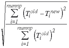
There are two or four values that are calculated to determine the quality of the convergence. The first value is the corrective norm. The corrective norm is calculated as:

where numnp is the total number of nodes in the model, T old is the temperature from the previous iteration, and T new is the iteration from the current iteration. This norm is related to the temperature difference between iterations; hence the name corrective norm.
The second value for the convergence is the relative norm. This is calculated as:
This norm is similar to the relative change in temperature between iterations; hence the name relative norm. The Corrective tolerance field can be used to define the maximum value for the corrective norm. The Relative tolerance field can be used to define the maximum value for the relative norm.
When the analysis includes body-to-body radiation, convergence is also based on heat flux; when the analysis includes phase change, convergence is also based on the liquid fraction. The equations for the corrective and relative norms based on heat flux or liquid fraction are the same as the above (replacing the temperatures with the heat fluxes or liquid fraction).
The temperature of a node after an iteration, T new , could be higher or lower than the final converged value. Thus, you may not want to use this value as the input for the next iteration. The value in the Relaxation parameter field can be used to minimize these oscillations. The relaxation parameter is used as follows:
T cur = T old + (relaxation parameter)*(T new - T old )
In a graphical format, the relationship between the different results can be shown as Figure 1. T cur , and therefore the effect of the relaxation parameter, is the value output to the results file.
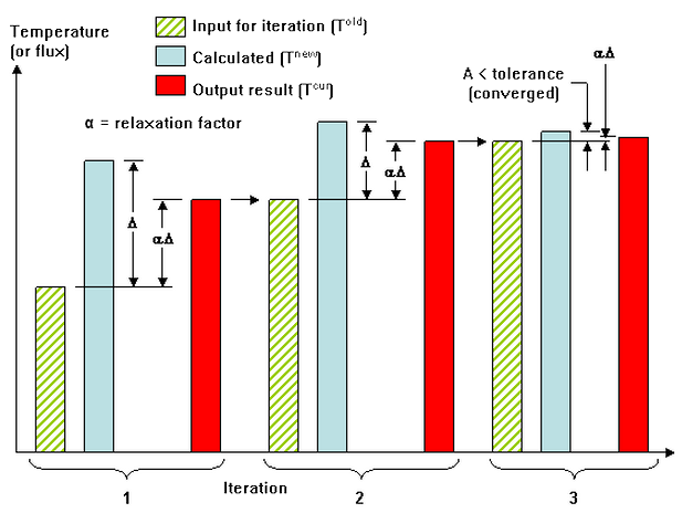
Figure 1: Graphical Interpretation of Relaxation Parameter
A relaxation parameter between 0.8 and 1 will provide good convergence when the nonlinear effects are small. When large nonlinear effects are present such as radiation at high temperatures the relaxation parameter may need to be on the order of 0.1 to 0.3 to smooth the oscillations. The convergence history can be checked in the log file.
- The convergence tolerances should be smaller than the expected change in result per time step (and perhaps significantly smaller to obtain accurate results). So in a model where iterations are needed only because of the temperatures, and if the smallest temperature change per time step is 10 degrees, a corrective tolerance of 0.1 degrees may be acceptable.
- Phase change is often a slow process, meaning that the change in the liquid fraction happens very slowly during the melting or freezing process. Therefore, if the change in the liquid fraction is only 0.01 per time step, then the corrective tolerance may need to be 0.0001 (or smaller) to get accurate results. A similar process can be applied to the relative tolerance.
- As always, review the log file during and after the analysis and check the convergence history. If the convergence criteria (corrective or relative norm) is large compared to the change in the result, then the solution may not be accurate.
Control Matrix Calculations
Some of the analysis time in a transient heat transfer analysis is spent creating the stiffness matrix at each time step. In some cases, this matrix does not need to be recalculated at every time step; reformulating it at every other time step may be sufficient (and save some calculation time). In a few cases, it is not necessary to update the matrix at all.
How often the matrix is recalculated is done using the Number of time steps between matrix reformulation field in the Advanced tab. The following factors require the matrix to be recalculated often (every step or every other step) to get accurate results:
- Radiation loads (both surface-based and body-to-body radiation)
- Phase change material model
- Temperature-dependent material properties
- Temperature-dependent loading
- Time dependent loading
- Variable time step size
If set to 0, the matrix is calculated at the beginning of the analysis and not updated thereafter.
Contact Options
There are two methods of handling bonded connections. Which method is used depends in part on whether the nodes are matched between the two parts or not matched.
Activating the option Enable smart bonded/welded contact will use multi-point constraint equations (MPCs) when necessary to bond the nodes on part A, surface B with the nearest nodes on part C, surface D. Shape functions interpolate the temperatures at the nodes on surface B to the nodes on surface D. Therefore, the meshes do not need to match between the parts. The MPCs are used for all the nodes on the surface contact pair whenever any node does not match. If the meshes do match at all nodes, then node matching will be used to bond the contact surface. The two vertices on the adjoining parts are collapsed to one node, and MPC equations are not used for the contacting surfaces. The options for the smart bonding drop-down are as follows:
- None: Smart bonding will not be used. Therefore, the nodes must match in order for parts to be bonded.
- Coarse bonded to fine mesh: Smart bonding will create MPC equations that connect the nodes on the surface with the coarser mesh to the nodes on the surface with the finer mesh.
- Fine bonded to coarse mesh: Smart bonding will create MPC equations that connect the nodes on the surface with the finer mesh to the nodes on the surface with the coarser mesh.
The smart bonding option applies to bonded contact and welded contact. Other types of contact (except for Free) require the nodes to be matched. (See the page Meshing Overview: Creating Contact Pairs: Types of Contact for a discussion of defining contact and using smart bonding.
By default, smart bonding uses the condensation method to solve your analysis. If you find your analysis doesn't converge or is not performing as you expect, you can try a different Solution method to use with MPC equations (see Multi-Point Constraints). Click Setup LoadsMulti-Point Constraint and choose from the Solution method options. If you use the Penalty Method, the accuracy of the solution is controlled by the Penalty multiplier field. The Penalty multiplier, times the maximum diagonal stiffness in the model, is used during the penalty solution. A value in the range of 10
4
to 10
6
is recommended.
LoadsMulti-Point Constraint and choose from the Solution method options. If you use the Penalty Method, the accuracy of the solution is controlled by the Penalty multiplier field. The Penalty multiplier, times the maximum diagonal stiffness in the model, is used during the penalty solution. A value in the range of 10
4
to 10
6
is recommended.
- The solution method you select in the Define Multi-Point Constraints dialog box becomes the method used for all features that include MPCs. These features include, but are not limited to, cyclic symmetry, frictionless constraints, smart bonding, and user-defined MPCs. For example, if you want to use the Penalty Method to solve all your analyses involving smart bonding, you can override the default condensation method by selecting Penalty Method in the Define Multi-Point Constraints dialog box.
- Smart bonding applied to contact between brick, 2D, and plate elements. Bonded contact involving other element types requires the nodes to match and are not affected by the smart bonding setting.
When the option Enable smart bonded/welded contact is not activated, the parts will be bonded only if the nodes match between the parts.