Wind loads simulation convergence

The wind simulation does not result in totally stable results as it is a dynamic process changing over time.

In order to address this problem, the program measures the resulting total forces convergence from one iteration to the next over a specific time period.

Deviation Factor

The deviation factor is used to identify when the solution has converged. As soon as the percentage of difference between two iterations falls below the deviation factor, the solution has converged.

Total Forces

The resultant forces are monitored in three directions:

• In the direction of the wind: .
• Horizontally and perpendicularly to the wind direction: .
• In the vertical direction: .

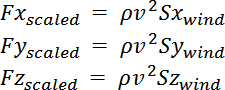
Scaling Forces

The resultant forces depend on the model size. To properly scale the resultant forces, the program uses the dynamic pressure and the surface values ,, and .

The surface values are used to scale the corresponding forces.

This approach allows for the neutralization of disproportions of the model in the wind directions x, y and z.

These relative values are calculated as follows:

• 
  Where:

  • represents the dynamic pressure in pascals.
  • represents the fluid density in kg/m³ .
  • represents the fluid velocity in m/s.
• The surface corresponds to the area covered by the projection of all the triangles of the model on the plane perpendicular to the X wind direction.
• The surface corresponds to the area covered by the projection of all the triangles of the model on the plane perpendicular to the Y wind direction.
• The surface corresponds to the area covered by the projection of all the triangles of the model on the plane perpendicular to the Z wind direction.

The scaling forces are calculated as follows:

Assessment of resultant forces stabilization

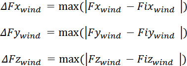
To measure the total forces convergence over a specific time period, the resultant forces , , and are calculated and stored for a number of steps n, and then the maximum change for a given moment is calculated as follows:

Where , , and represent the stored values of , , and for a given step, and for i=1 to n.

These maximum force changes are then scaled by , , and respectively and displayed as a percentage.

The final metric is the maximum of these three scaled values:

Where = 0,5%, i.e. the default load deviation factor.

Note: In order for the metric to be fully valid, at least n steps of the simulation must be performed.

n is the number of simulation steps for which , , and are stored for comparison with the current step. The default value for n is 10.