Material Characterization

There are two approaches to material characterization available for use in Advanced Material Exchange: Multi-Layer and Single-Layer. Each approach can be used to determine the Elastic and Plastic Coefficients, the failure coefficients, and the compression stress drop coefficients (if compressive data is provided).

Multi-Layer

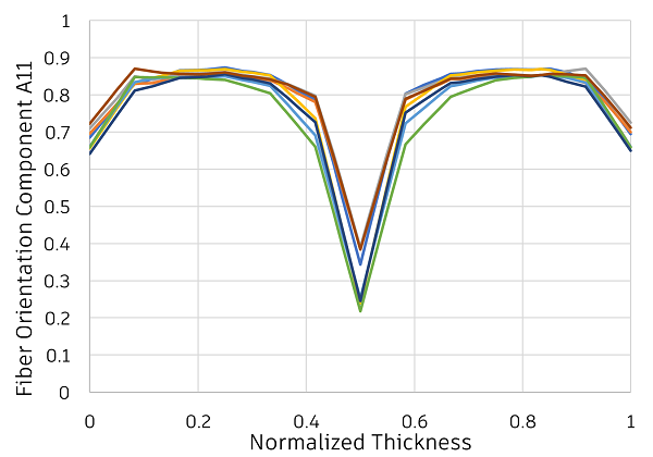
The fiber orientation tensor varies widely through the thickness of a part. The image below shows an example of how the A11 component of the fiber orientation tensor varies through the thickness of a model for several materials. The other components, not shown, also vary through the thickness.

To capture the variance in the fiber distribution through the thickness, we must apply more than one fiber orientation tensor. This leads us to the Multi-Layer approach, which is the default material characterization method used in Advanced Material Exchange. The Multi-Layer approach is built on Classic Lamination Theory (CLT) [16]. With this approach, there are twelve layers through the thickness of the material (or six layers in a half-symmetry model). Each layer has a unique fiber orientation tensor, allowing us to capture a more realistic representation of the fiber distribution through the thickness.

In observed results using the Moldflow Rotational Diffusion model, there is a strong correlation between the fiber orientation tensor predictions and the fiber volume fraction of the material. Given this dependence, the fiber volume fraction is used in a polynomial fit to generate the through-thickness orientations for each layer. First, the fiber orientation tensor is determined on the surface layer. Next, the fiber orientation tensor is determined in the center (6th) layer. The fiber orientation tensors for the remaining four layers in between the surface and the center are determined using linear interpolation.

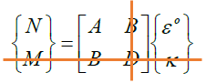
The Multi-Layer method assumes there is no coupling between the force and curvatures.

where

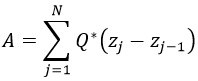
Q** represents the plane stress stiffness matrix and *zj -z j-1 represents the thickness of each layer.

Using this approach, a load is applied incrementally to the Multi-Layer model to determine the set of elastic and plastic coefficients that best fit the experimental data.

Polynomial Stress Failure Coefficients

The failure coefficients used to evaluate rupture with the Polynomial Stress rupture criteria vary depending on the largest eigenvalue of the fiber orientation tensor at each integration point in the model. As a result, several sets of these coefficients (A11m, A22m, A33m, A12m, A13m, and A23m) must be determined during the material characterization routine in order to span the possible range of the largest eigenvalue.

To start, each layer in the CLT model is loaded individually with the load applied at 0, 45, and 90 degrees to the material coordinate system. At this point, we can extract the maximum strain at failure for each angle of loading. Using these maximum strain values, we can exercise the material model over a range of fiber orientation tensors. This gives us unique matrix stresses across the range of fiber orientation tensors. These stresses are used to solve a system of equations and calculate the failure coefficients.

MCT Failure Coefficients

The failure coefficients A1m, A2m, and A4m for the MCT rupture criteria are also determined during the material characterization routine.

To start, the CLT model is run to the maximum strain value for each of the 3 experimental stress-strain curves (0, 90, and 45 degree data sets). If you don’t have stress-strain data at 45 degrees, we use the 90 degree curve and raise the stress data points by 5%. At this point we can gather the matrix stresses for the center layer of the CLT model. By solving the system of equations, we arrive at an initial guess for A1m, A2m, and A4m.

Our goal is to produce a set of failure coefficients that correctly predict first ply failure for the 0, 90, and 45 degree load cases. Therefore, we operate on the initial guess for A1m, A2m, and A4m to produce a bounded range. The range is simply computed as Aim ± abs(Aim). Next, a Monte Carlo simulation with a sample size of 300,000 is performed to produce a random sets of A1m, A2m, and A4m within these bounds for the case of a unidirectional fiber.

Now we cycle through each random set and perform fiber orientation averaging on the three failure coefficients for each layer in the CLT model. We can compute the error produced by the CLT model in relation to first ply failure as FI - 1, where FI is the failure index. This error computation is performed for each of the three curves (0, 90, and 45 degrees).

Finally, the total error is computed as the sum of each individual error computation. Now we can select the random set of failure coefficients that minimizes the error. This gives us the final set of failure coefficients.

Single-Layer

The Single-Layer material characterization scheme assumes a constant value for the fiber orientation tensor through the thickness of the material. In reality, the fiber orientation tensor varies widely through the thickness of a part. This is one of the drawbacks to using the Single-Layer material characterization scheme.

The Single-Layer material characterization scheme has the advantage of being faster than the default Multi-Layer routine described above. Since there is only a single fiber orientation tensor to consider, the material characterization is quicker. The Single-Layer scheme may be useful if you used something other than the Moldflow Rotational Diffusion model to predict fiber orientation tensors in Moldflow. If you used the Moldflow Rotational Diffusion model, we recommend you use the default Multi-Layer method described above, which is designed for use with the Moldflow Rotational Diffusion model.

If you use the MCT or Maximum Effective Stress rupture criteria, the Single-Layer material characterization scheme can be used to determine the failure coefficients, but we recommend the use of the Multi-Layer scheme. The Multi-Layer scheme captures the more of the through-thickness variance in rupture predictions.