The Rupture Model

The plasticity response of the matrix constituent material is defined collectively by Eqs. 1-8. However, the model must also utilize a rupture criterion that identifies complete failure of the short fiber filled material. There are three rupture criteria available for use with Advanced Material Exchange.

Polynomial Stress

The Polynomial Stress method is the default rupture model used by Advanced Material Exchange. In the Polynomial Stress method, we assume the matrix rupture criterion is a quadratic function of the matrix average stress components.

The quantities (i = 11, 22, 33, 12, 13, 23) are the adjustable coefficients of the matrix failure criteria that must be determined from tensile tests for the 0, 90, and 45 degree data sets. If you don't have stress-strain data at 45 degrees, we use the 90 degree curve and raise the stress data points by 5%. Refer to the Material Characterization topic for more details on how the failure coefficients are determined.

The set of failure coefficients used to evaluate rupture varies depending on the largest eigenvalue of the fiber orientation tensor at each integration point in the model. When the largest eigenvalue is > 0.65, we assume a transversely isotropic behavior so that σ22m = σ33m and σ12m = σ13m. We also assume the out of plane shear stress component σ23m = σ12m = σ13m. Accordingly, A22 = A33 and A12 = A13 = A23.

When the largest eigenvalue is ≤ 0.65, we assume an isotropic behavior so that σ11m = σ22m = σ33m and σ12m = σ13m = σ23m. Accordingly, A11 = A22 = A33 and A12 = A13 = A23.

MCT

In the MCT method, we assume the matrix rupture criterion is expressed as a quadratic function of the matrix average stress components.

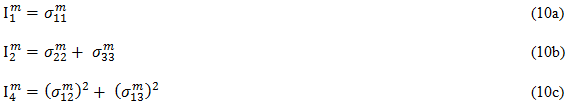
In Eq. 9, the quantities (j = 1, 2, 4) are transversely isotropic invariants of the matrix average stress state.

The quantities (i = 1, 2, 4) are the adjustable coefficients of the matrix failure criteria that must be determined from tensile tests for the 0, 90, and 45 degree data sets. If you don't have stress-strain data at 45 degrees, we use the 90 degree curve and raise the stress data points by 5%. Refer to the Material Characterization topic for more details on how the failure coefficients are determined.

Maximum Effective Stress

In the Maximum Effective Stress rupture model, we assume the functional form of the effective stress expression (a weighted von Mises stress, see Eq. 6) is sufficient to define the directional dependency of the material for both the prediction of matrix plastic evolution and the prediction of matrix rupture. Therefore, the determination of the matrix rupture criterion requires that we simply establish an upper limit on the value of the weighted effective stress measure (denoted the effective strength Seff). In this case, the matrix rupture criterion is expressed as

where it is understood that the stress components represent the average stress in the matrix constituent material.

Damage Evolution

Once the matrix rupture condition is satisfied (either MCT or Maximum Effective Stress), several changes are made to the constitutive relations of the failed material.

1. There is no longer any need to decompose the composite stress and strain into matrix stress and strain since we no longer have to compute plastic evolution for the matrix.
2. The constitutive relations of the homogenized composite material are used directly instead of building the composite constitutive relations from the constituent constitutive relations and microstructure (as seen earlier).
3. The stiffness of the composite material is instantaneously reduced to a fraction of the original elastic stiffness of the composite material. This stiffness reduction is performed by multiplying the stiffness matrix by a degradation constant. Note, once the rupture condition is triggered, the stiffness of the composite material remains fixed at the reduced value for the duration of the simulation.
4. The composite constitutive relations are switched from a tangent formulation (which was used during the plasticity phase of the material response) to a secant formulation. Since the stiffness of the failed composite material remains fixed, the integration point in question no longer makes any direct contribution to the nonlinearity of the solution.